
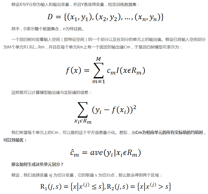
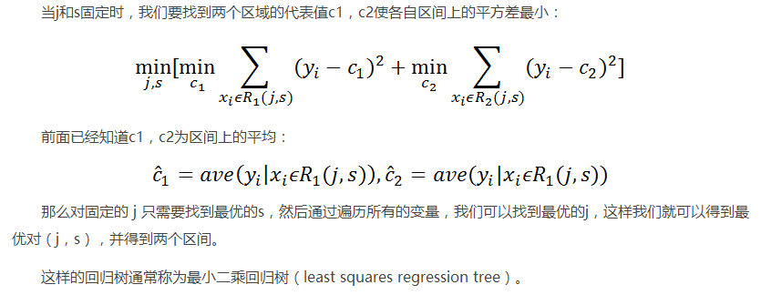
機器學習實戰(九)樹迴歸
第九章 樹迴歸
第三章使用決策樹進行分類,其不斷將資料切分為小資料,直到目標變數完全相同,或者資料不能再分為止,決策樹是一種貪心演算法,要在給定的時間內做出最佳選擇,但並不關心能否達到全域性最優。
9.1 CART(Classification And Regression Trees)演算法用於迴歸


CART演算法:
CART演算法正好適用於連續型特徵。CART演算法使用二元切分法來處理連續型變數。而使用二元切分法則易於對樹構建過程進行調整以處理連續型特徵。具體的處理方法是:如果特徵值大於給定值就走左子樹,否則就走右子樹。
CART演算法有兩步:
- 決策樹生成:遞迴地構建二叉決策樹的過程,基於訓練資料集生成決策樹,生成的決策樹要儘量大;自上而下從根開始建立節點,在每個節點處要選擇一個最好的屬性來分裂,使得子節點中的訓練集儘量的純。不同的演算法使用不同的指標來定義”最好”:
- 決策樹剪枝:用驗證資料集對已生成的樹進行剪枝並選擇最優子樹,這時損失函式最小作為剪枝的標準。
決策樹剪枝我們先不管,我們看下決策樹生成。
在決策樹的文章中,我們先根據資訊熵的計算找到最佳特徵切分資料集構建決策樹。CART演算法的決策樹生成也是如此,實現過程如下:
- 使用CART演算法選擇特徵
- 根據特徵切分資料集合
- 構建樹
根據特徵切分資料集合。編寫程式碼如下:
import numpy as np
def binSplitDataSet(dataSet, feature, value):
"""
根據特徵切分資料集合
:param dataSet: 資料集合
:param feature: 帶切分的特徵
:param value: 該特徵的值
:return:
mat0:切分的資料集合0
mat1:切分的資料集合1
""" 結果:

根據是否大於0.5的規則進行切分
9.1.1 用CART演算法選擇最佳分類特徵
防止過擬合:
tolS:控制誤差變化限制tolN:切分特徵最少樣本數
上述兩個引數是為了防止過擬合,提前設定終止條件,實際上是在進行一種所謂的預剪枝。
一、資料集視覺化程式碼:
資料集:ex00.txt
import matplotlib.pyplot as plt
import numpy as np

def loadDataSet(fileName):
    """
    函式說明:載入資料
    Parameters:
        fileName - 檔名
    Returns:
        dataMat - 資料矩陣

    """
    dataMat = []
    fr = open(fileName)
    for line in fr.readlines():
        curLine = line.strip().split('\t')
        fltLine = list(map(float, curLine))                    #轉化為float型別
        dataMat.append(fltLine)
    return dataMat

def plotDataSet(filename):
    """
    函式說明:繪製資料集
    Parameters:
        filename - 檔名
    Returns:
        無

    """
    dataMat = loadDataSet(filename)                                        #載入資料集
    n = len(dataMat)                                                    #資料個數
    xcord = []; ycord = []                                                #樣本點
    for i in range(n):
        xcord.append(dataMat[i][0]); ycord.append(dataMat[i][1])        #樣本點
    fig = plt.figure()
    ax = fig.add_subplot(111)                                            #新增subplot
    ax.scatter(xcord, ycord, s = 20, c = 'blue',alpha = .5)                #繪製樣本點
    plt.title('DataSet')                                                #繪製title
    plt.xlabel('X')
    plt.show()

if __name__ == '__main__':
    filename = 'ex00.txt'
    plotDataSet(filename)
結果:

二、利用該資料集測試CART演算法程式碼
#-*- coding:utf-8 -*-
import numpy as np

def loadDataSet(fileName):
    """
    函式說明:載入資料
    Parameters:
        fileName - 檔名
    Returns:
        dataMat - 資料矩陣
    """
    dataMat = []
    fr = open(fileName)
    for line in fr.readlines():
        curLine = line.strip().split('\t')
        fltLine = list(map(float, curLine))                    #轉化為float型別
        dataMat.append(fltLine)
    return dataMat

def binSplitDataSet(dataSet, feature, value):
    """
    函式說明:根據特徵切分資料集合
    Parameters:
        dataSet - 資料集合
        feature - 帶切分的特徵
        value - 該特徵的值
    Returns:
        mat0 - 切分的資料集合0
        mat1 - 切分的資料集合1

    """
    mat0 = dataSet[np.nonzero(dataSet[:,feature] > value)[0],:]
    mat1 = dataSet[np.nonzero(dataSet[:,feature] <= value)[0],:]
    return mat0, mat1
def regLeaf(dataSet):
    """
    函式說明:生成葉結點
    Parameters:
        dataSet - 資料集合
    Returns:
        目標變數的均值

    """
    return np.mean(dataSet[:,-1])
def regErr(dataSet):
    """
    函式說明:誤差估計函式
    Parameters:
        dataSet - 資料集合
    Returns:
        目標變數的總方差
    """
    return np.var(dataSet[:,-1]) * np.shape(dataSet)[0]

def chooseBestSplit(dataSet, leafType = regLeaf, errType = regErr, ops = (1,4)):
    """
    函式說明:找到資料的最佳二元切分方式函式
    Parameters:
        dataSet - 資料集合
        leafType - 生成葉結點
        regErr - 誤差估計函式
        ops - 使用者定義的引數構成的元組
    Returns:
        bestIndex - 最佳切分特徵
        bestValue - 最佳特徵值
    """
    import types
    #tolS允許的誤差下降值,tolN切分的最少樣本數
    tolS = ops[0]; tolN = ops[1]
    #如果當前所有值相等,則退出。(根據set的特性)
    if len(set(dataSet[:,-1].T.tolist()[0])) == 1:
        return None, leafType(dataSet)
    #統計資料集合的行m和列n
    m, n = np.shape(dataSet)
    #預設最後一個特徵為最佳切分特徵,計算其誤差估計
    S = errType(dataSet)
    #分別為最佳誤差,最佳特徵切分的索引值,最佳特徵值
    bestS = float('inf'); bestIndex = 0; bestValue = 0
    #遍歷所有特徵列
    for featIndex in range(n - 1):
        #遍歷所有特徵值
        for splitVal in set(dataSet[:,featIndex].T.A.tolist()[0]):
            #根據特徵和特徵值切分資料集
            mat0, mat1 = binSplitDataSet(dataSet, featIndex, splitVal)
            #如果資料少於tolN,則退出
            if (np.shape(mat0)[0] < tolN) or (np.shape(mat1)[0] < tolN): continue
            #計算誤差估計
            newS = errType(mat0) + errType(mat1)
            #如果誤差估計更小,則更新特徵索引值和特徵值
            if newS < bestS:
                bestIndex = featIndex
                bestValue = splitVal
                bestS = newS
    #如果誤差減少不大則退出
    if (S - bestS) < tolS:
        return None, leafType(dataSet)
    #根據最佳的切分特徵和特徵值切分資料集合
    mat0, mat1 = binSplitDataSet(dataSet, bestIndex, bestValue)
    #如果切分出的資料集很小則退出
    if (np.shape(mat0)[0] < tolN) or (np.shape(mat1)[0] < tolN):
        return None, leafType(dataSet)
    #返回最佳切分特徵和特徵值
    return bestIndex, bestValue

if __name__ == '__main__':
    myDat = loadDataSet('ex00.txt')
    myMat = np.mat(myDat)
    feat, val = chooseBestSplit(myMat, regLeaf, regErr, (1, 4))
    print(feat)
    print(val)
結果:
0
0.48813
分析:
切分的最佳特徵為第一列特徵,最佳切分特徵值為0.48813
選擇標準:選取使得誤差最小化的特徵
9.1.2 利用所選的兩個變數建立迴歸樹
import numpy as np

def loadDataSet(fileName):
    """
    函式說明:載入資料
    Parameters:
        fileName - 檔名
    Returns:
        dataMat - 資料矩陣

    """
    dataMat = []
    fr = open(fileName)
    for line in fr.readlines():
        curLine = line.strip().split('\t')
        fltLine = list(map(float, curLine))                    #轉化為float型別
        dataMat.append(fltLine)
    return dataMat

def binSplitDataSet(dataSet, feature, value):
    """
    函式說明:根據特徵切分資料集合
    Parameters:
        dataSet - 資料集合
        feature - 帶切分的特徵
        value - 該特徵的值
    Returns:
        mat0 - 切分的資料集合0
        mat1 - 切分的資料集合1
    Website:
        http://www.cuijiahua.com/
    Modify:
        2017-12-12
    """
    mat0 = dataSet[np.nonzero(dataSet[:,feature] > value)[0],:]
    mat1 = dataSet[np.nonzero(dataSet[:,feature] <= value)[0],:]
    return mat0, mat1

def regLeaf(dataSet):
    """
    函式說明:生成葉結點
    Parameters:
        dataSet - 資料集合
    Returns:
        目標變數的均值

    """
    return np.mean(dataSet[:,-1])

def regErr(dataSet):
    """
    函式說明:誤差估計函式
    Parameters:
        dataSet - 資料集合
    Returns:
        目標變數的總方差

    """
    return np.var(dataSet[:,-1]) * np.shape(dataSet)[0]

def chooseBestSplit(dataSet, leafType = regLeaf, errType = regErr, ops = (1,4)):
    """
    函式說明:找到資料的最佳二元切分方式函式
    Parameters:
        dataSet - 資料集合
        leafType - 生成葉結點
        regErr - 誤差估計函式
        ops - 使用者定義的引數構成的元組
    Returns:
        bestIndex - 最佳切分特徵
        bestValue - 最佳特徵值

    """
    import types
    #tolS允許的誤差下降值,tolN切分的最少樣本數
    tolS = ops[0]; tolN = ops[1]
    #如果當前所有值相等,則退出。(根據set的特性)
    if len(set(dataSet[:,-1].T.tolist()[0])) == 1:
        return None, leafType(dataSet)
    #統計資料集合的行m和列n
    m, n = np.shape(dataSet)
    #預設最後一個特徵為最佳切分特徵,計算其誤差估計
    S = errType(dataSet)
    #分別為最佳誤差,最佳特徵切分的索引值,最佳特徵值
    bestS = float('inf'); bestIndex = 0; bestValue = 0
    #遍歷所有特徵列
    for featIndex in range(n - 1):
        #遍歷所有特徵值
        for splitVal in set(dataSet[:,featIndex].T.A.tolist()[0]):
            #根據特徵和特徵值切分資料集
            mat0, mat1 = binSplitDataSet(dataSet, featIndex, splitVal)
            #如果資料少於tolN,則退出
            if (np.shape(mat0)[0] < tolN) or (np.shape(mat1)[0] < tolN): continue
            #計算誤差估計
            newS = errType(mat0) + errType(mat1)
            #如果誤差估計更小,則更新特徵索引值和特徵值
            if newS < bestS:
                bestIndex = featIndex
                bestValue = splitVal
                bestS = newS
    #如果誤差減少不大則退出
    if (S - bestS) < tolS:
        return None, leafType(dataSet)
    #根據最佳的切分特徵和特徵值切分資料集合
    mat0, mat1 = binSplitDataSet(dataSet, bestIndex, bestValue)
    #如果切分出的資料集很小則退出
    if (np.shape(mat0)[0] < tolN) or (np.shape(mat1)[0] < tolN):
        return None, leafType(dataSet)
    #返回最佳切分特徵和特徵值
    return bestIndex, bestValue

def createTree(dataSet, leafType = regLeaf, errType = regErr, ops = (1, 4)):
    """
    函式說明:樹構建函式
    Parameters:
        dataSet - 資料集合
        leafType - 建立葉結點的函式
        errType - 誤差計算函式
        ops - 包含樹構建所有其他引數的元組
    Returns:
        retTree - 構建的迴歸樹

    """
    #選擇最佳切分特徵和特徵值
    feat, val = chooseBestSplit(dataSet, leafType, errType, ops)
    #r如果沒有特徵,則返回特徵值
    if feat == None: return val
    #迴歸樹
    retTree = {}
    retTree['spInd'] = feat
    retTree['spVal'] = val
    #分成左資料集和右資料集
    lSet, rSet = binSplitDataSet(dataSet, feat, val)
    #建立左子樹和右子樹
    retTree['left'] = createTree(lSet, leafType, errType, ops)
    retTree['right'] = createTree(rSet, leafType, errType, ops)
    return retTree

if __name__ == '__main__':
    myDat = loadDataSet('ex00.txt')
    myMat = np.mat(myDat)
    print(createTree(myMat))
結果:
{'spVal': 0.48813, 'right': -0.044650285714285719, 'spInd': 0,
'left': 1.0180967672413792}
分析:
該樹只有兩個葉結點。
利用複雜資料進行實驗:
資料集:ex0.txt
import matplotlib.pyplot as plt
import numpy as np

def loadDataSet(fileName):
    """
    函式說明:載入資料
    Parameters:
        fileName - 檔名
    Returns:
        dataMat - 資料矩陣

    """
    dataMat = []
    fr = open(fileName)
    for line in fr.readlines():
        curLine = line.strip().split('\t')
        fltLine = list(map(float, curLine))                    #轉化為float型別
        dataMat.append(fltLine)
    return dataMat

def plotDataSet(filename):
    """
    函式說明:繪製資料集
    Parameters:
        filename - 檔名
    Returns:
        無

    """
    dataMat = loadDataSet(filename)                                        #載入資料集
    n = len(dataMat)                                                    #資料個數
    xcord = []; ycord = []                                                #樣本點
    for i in range(n):
        xcord.append(dataMat[i][1]); ycord.append(dataMat[i][2])        #樣本點
    fig = plt.figure()
    ax = fig.add_subplot(111)                                            #新增subplot
    ax.scatter(xcord, ycord, s = 20, c = 'blue',alpha = .5)                #繪製樣本點
    plt.title('DataSet')                                                #繪製title
    plt.xlabel('X')
    plt.show()

if __name__ == '__main__':
    filename = 'ex0.txt'
    plotDataSet(filename)
結果:

9.2 樹剪枝
一棵樹如果結點過多,表明該模型可能對資料進行了“過擬合”,如何判斷是否過擬合,前面已經介紹了使用測試集上的某種交叉驗證的方法來發現過擬合,決策樹一樣。
通過降低樹的複雜度來避免過擬合的過程稱為剪枝(pruning)。我們也已經提到,設定tolS和tolN就是一種預剪枝操作。另一種形式的剪枝需要使用測試集和訓練集,稱作後剪枝(postpruning)。本節將分析後剪枝的有效性,但首先來看一下預剪枝的不足之處。
9.2.1 預剪枝
利用ex2.txt實驗結果:

雖然和上圖很相似,但是y的數量級差了很多倍,資料分佈相似,但是構建出的樹有很多葉結點。產生這個現象的原因在於,停止條件tolS對誤差的數量級十分敏感。如果在選項中花費時間並對上述誤差容忍度取平均值,或許也能得到僅有兩個葉結點組成的樹,可以看到,將引數tolS修改為10000後,構建的樹就是隻有兩個葉結點。然而,顯然這個值,需要我們經過不斷測試得來,顯然通過不斷修改停止條件來得到合理結果並不是很好的辦法。事實上,我們常常甚至不確定到底需要尋找什麼樣的結果。因為對於一個很多維度的資料集,你也不知道構建的樹需要多少個葉結點。
可見,預剪枝有很大的侷限性。接下來,我們討論後剪枝,即利用測試集來對樹進行剪枝。由於不需要使用者指定引數,後剪枝是一個更理想化的剪枝方法。
9.2.2 後剪枝
使用後剪枝方法需要將資料集分成測試集和訓練集。首先指定引數,使得構建出的樹足夠大、足夠複雜,便於剪枝。接下來從上而下找到葉結點,用測試集來判斷這些葉結點合併是否能降低測試集誤差。如果是的話就合併。後剪枝可能不如預剪枝有效。一般地,為了尋求最佳模型可以同時使用兩種剪枝技術。
9.3 模型樹
用樹來對資料建模,除了把葉節點簡單的設定為常數值外,還有一種方法是把葉節點設定為分段線性函式,即模型由多個線性片段組成。
很顯然,兩條直線比很多節點組成的一棵大樹更容易解釋。

考慮圖9-4中的資料。如果使用兩條直線擬合是否比使用一組常數來建模好呢?答案顯而易見。可以設計兩條分別從0.0~0.3、從0.3~1.0的直線,於是就可以得到兩個線性模型。因為資料集裡的一部分資料(0.0~0.3)以某個線性模型建模,而另一部分資料(0.3~1.0)則以另一個線性模型建模,因此我們說採用了所謂的分段線性模型。
模型樹的優於迴歸樹的優點:
1)可解釋性
2)有更高的預測準確度
下面將利用樹生成演算法對資料進行切分,且每份切分資料都能很容易被線性模型所表示。
該演算法的關鍵在於誤差的計算,應該怎樣計算誤差呢?
前面用於迴歸樹的誤差計算方法這裡不能再用。稍加變化,對於給定的資料集,應該先用線性的模型來對它進行擬合,然後計算真實的目標值與模型預測值間的差值。最後將這些差值的平方求和就得到了所需的誤差。
9.3 總結
1)CART演算法可以用於構建二元樹並處理離散型或連續型資料的切分。若使用不同的誤差準則,就可以通過CART演算法構建模型樹和迴歸樹。
2)一顆過擬合的樹常常十分複雜,剪枝技術的出現就是為了解決這個問題。兩種剪枝方法分別是預剪枝和後剪枝,預剪枝更有效但需要使用者定義一些引數。