
基於卷積神經網路特徵圖的二值影象分割
目標檢測是當前大火的一個研究方向,FasterRCNN、Yolov3等一系列結構也都在多目標檢測的各種應用場景或者競賽中取得了很不錯的成績。但是想象一下,假設我們需要通過影象檢測某個產品上是否存在缺陷,或者通過衛星圖判斷某片海域是否有某公司的船隻,再或者需要研發一套無人駕駛中基於影象的避障裝置。這些問題的共同特點是,我們只需要檢測出某種特定目標在圖片中的位置,並不需要在同一幅圖中識別出多個目標。這種時候,FasterRCNN或者Yolov3等演算法當然完全能夠勝任,但是多少有些殺雞用牛刀的感覺,因為考慮到這些網路需要相對較多的計算資源。當我們僅僅需要檢測某一類特定目標的話,我們更希望網路能夠專注於學習到那一個特定目標的特徵。15年所提出的U-net網路正是通過多個多通道特徵圖最大化的利用輸入圖片的特徵,以實現目標的二值影象分割,並在kaggle上的各類影象分割相關賽事中被廣泛使用。U-net論文:
這裡僅建立一個比較簡單的網路模型,來對基於卷積神經網路特徵圖的二值影象分割方法進行說明。網路基於keras建立,結構如下:
def Conv2d_BN(x, nb_filter, kernel_size, strides=(1,1), padding='same'):
    x = Conv2D(nb_filter, kernel_size, strides=strides, padding=padding)(x)
    x = BatchNormalization(axis=3)(x)
    x = LeakyReLU(alpha=0.1)(x)
    return x

def Conv2dT_BN(x, filters, kernel_size, strides=(2,2), padding='same'):
    x = Conv2DTranspose(filters, kernel_size, strides=strides, padding=padding)(x)
    x = BatchNormalization(axis=3)(x)
    x = LeakyReLU(alpha=0.1)(x)
    return x

inpt = Input(shape=(input_size_1, input_size_2, 3))
x = Conv2d_BN(inpt, 4, (3, 3))
x = MaxPooling2D(pool_size=(3,3),strides=(2,2),padding='same')(x)
x = Conv2d_BN(x, 8, (3, 3))
x = MaxPooling2D(pool_size=(3,3),strides=(2,2),padding='same')(x)
x = Conv2d_BN(x, 16, (3, 3))
x = AveragePooling2D(pool_size=(3,3),strides=(2,2),padding='same')(x)
x = Conv2d_BN(x, 32, (3, 3))
x = AveragePooling2D(pool_size=(3,3),strides=(2,2),padding='same')(x)
x = Conv2d_BN(x, 64, (3, 3))
x = Dropout(0.5)(x)
x = Conv2d_BN(x, 64, (1, 1))
x = Dropout(0.5)(x)
x = Conv2dT_BN(x, 32, (3, 3))
x = Conv2dT_BN(x, 16, (3, 3))
x = Conv2dT_BN(x, 8, (3, 3))
x = Conv2dT_BN(x, 4, (3, 3))

x = Conv2DTranspose(filters=3,kernel_size=(3,3),strides=(1,1),padding='same',activation='sigmoid')(x)

model = Model(inpt, x)
model.summary()
網路輸入的圖片大小為256*256*3。這樣搭起來的網路,只有50000+引數,如果是實際應用的話,再優化一下放到移動裝置裡邊實時性應該還是沒問題的。
由於網路輸出的二值影象分割結果尺寸應該和原始圖片保持一致,因此在網路使用了池化層對圖片進行壓縮之後,需要進行上取樣來對圖片的尺寸進行還原。一般而言,神經網路中常用的上取樣操作是up pooling或者轉置卷積,插值的話比較少見。個人覺得轉置卷積的效果會優於up pooling。網路使用最大值池化層來突出原始影象的邊緣特徵,同時均值池化層用來保留影象中的位置特徵,Dropout層加入噪聲防止過擬合。卷積層與反捲積層基本呈對稱結構,來方便對訓練集標籤進行更為自然的學習。
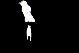
網路訓練與測試所使用的資料集,是在網上找到一些無異物的鐵路影象作為背景,同時基於VOC2012資料集中的圖片以及其提供的SegmentationObject標籤,將目標物體隨機縮放、旋轉後,與背景鐵路影象隨機組合生成偽造資料。資料集和標籤大概長下面這樣:
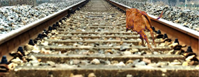
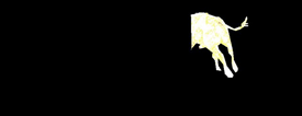


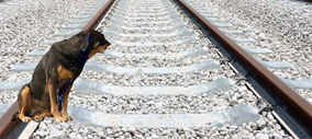

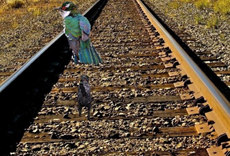
生成的訓練集和測試集各包含1000張圖片,訓練集與測試集放置的目標物體不同,訓練10個Epoch。訓練之後的網路對測試集的分類效果如下:
原始影象 真實標籤 檢測標籤
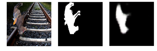


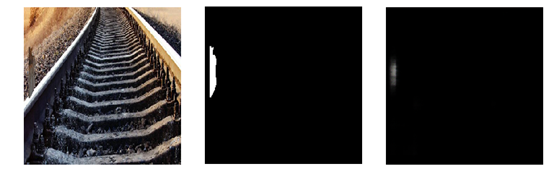
可以看出,即便是在限制條件較多的情況下,網路也能夠取得較好的檢測效果。對於測試集最後一張圖的小目標,網路檢測結果稍差,一方面是因為訓練集較小,訓練不完全的緣故,但也有網路容量本身的問題。在需要進行精度更高的檢測的情況下,可以適當將網路擴大或加深,簡單的將網路各層中卷積單元數量同時增加相同倍數就能得到更加好的結果,但相應的計算速度會有所下降。
當然,偽造資料集最大的問題在於背景多樣性不足,可能在背景更加複雜的情況下,所需要的網路容量也相應會更大。
網路使用的完整程式碼如下,資料讀取寫的比較囉嗦,反正就那麼個意思:
import numpy as np
import random
import os

from keras.models import save_model, load_model, Model
from keras.layers import Input, Dropout, BatchNormalization, LeakyReLU
from keras.layers import Conv2D, MaxPooling2D, AveragePooling2D, Conv2DTranspose
import matplotlib.pyplot as plt
from skimage import io
from skimage.transform import resize

input_name = os.listdir('train_data3/JPEGImages')

n = len(input_name)
batch_size = 8
input_size_1 = 256
input_size_2 = 256

"""
Batch_data
"""
def batch_data(input_name, n, batch_size = 8, input_size_1 = 256, input_size_2 = 256):
    rand_num = random.randint(0, n-1)
    img1 = io.imread('train_data3/JPEGImages/'+input_name[rand_num]).astype("float")
    img2 = io.imread('train_data3/TargetImages/'+input_name[rand_num]).astype("float")
    img1 = resize(img1, [input_size_1, input_size_2, 3])
    img2 = resize(img2, [input_size_1, input_size_2, 3])
    img1 = np.reshape(img1, (1, input_size_1, input_size_2, 3))
    img2 = np.reshape(img2, (1, input_size_1, input_size_2, 3))
    img1 /= 255
    img2 /= 255
    batch_input = img1
    batch_output = img2
    for batch_iter in range(1, batch_size):
        rand_num = random.randint(0, n-1)
        img1 = io.imread('train_data3/JPEGImages/'+input_name[rand_num]).astype("float")
        img2 = io.imread('train_data3/TargetImages/'+input_name[rand_num]).astype("float")
        img1 = resize(img1, [input_size_1, input_size_2, 3])
        img2 = resize(img2, [input_size_1, input_size_2, 3])
        img1 = np.reshape(img1, (1, input_size_1, input_size_2, 3))
        img2 = np.reshape(img2, (1, input_size_1, input_size_2, 3))
        img1 /= 255
        img2 /= 255
        batch_input = np.concatenate((batch_input, img1), axis = 0)
        batch_output = np.concatenate((batch_output, img2), axis = 0)
    return batch_input, batch_output

def Conv2d_BN(x, nb_filter, kernel_size, strides=(1,1), padding='same'):
    x = Conv2D(nb_filter, kernel_size, strides=strides, padding=padding)(x)
    x = BatchNormalization(axis=3)(x)
    x = LeakyReLU(alpha=0.1)(x)
    return x

def Conv2dT_BN(x, filters, kernel_size, strides=(2,2), padding='same'):
    x = Conv2DTranspose(filters, kernel_size, strides=strides, padding=padding)(x)
    x = BatchNormalization(axis=3)(x)
    x = LeakyReLU(alpha=0.1)(x)
    return x

inpt = Input(shape=(input_size_1, input_size_2, 3))
x = Conv2d_BN(inpt, 4, (3, 3))
x = MaxPooling2D(pool_size=(3,3),strides=(2,2),padding='same')(x)
x = Conv2d_BN(x, 8, (3, 3))
x = MaxPooling2D(pool_size=(3,3),strides=(2,2),padding='same')(x)
x = Conv2d_BN(x, 16, (3, 3))
x = AveragePooling2D(pool_size=(3,3),strides=(2,2),padding='same')(x)
x = Conv2d_BN(x, 32, (3, 3))
x = AveragePooling2D(pool_size=(3,3),strides=(2,2),padding='same')(x)
x = Conv2d_BN(x, 64, (3, 3))
x = Dropout(0.5)(x)
x = Conv2d_BN(x, 64, (1, 1))
x = Dropout(0.5)(x)
x = Conv2dT_BN(x, 32, (3, 3))
x = Conv2dT_BN(x, 16, (3, 3))
x = Conv2dT_BN(x, 8, (3, 3))
x = Conv2dT_BN(x, 4, (3, 3))

x = Conv2DTranspose(filters=3,kernel_size=(3,3),strides=(1,1),padding='same',activation='sigmoid')(x)

model = Model(inpt, x)
model.summary()

model.compile(loss='mean_squared_error', optimizer='Nadam', metrics=['accuracy'])

itr = 1000
S = []
for i in range(itr):
    print("iteration = ", i+1)
    if i < 500:
        bs = 4
    elif i < 2000:
        bs = 8
    elif i < 5000:
        bs = 16
    else:
        bs = 32
    train_X, train_Y = batch_data(input_name, n, batch_size = bs)
    model.fit(train_X, train_Y, epochs=1, verbose=0)

def batch_data_test(input_name, n, batch_size = 8, input_size_1 = 256, input_size_2 = 256):
    rand_num = random.randint(0, n-1)
    img1 = io.imread('test_data3/JPEGImages/'+input_name[rand_num]).astype("float")
    img2 = io.imread('test_data3/TargetImages/'+input_name[rand_num]).astype("float")
    img1 = resize(img1, [input_size_1, input_size_2, 3])
    img2 = resize(img2, [input_size_1, input_size_2, 3])
    img1 = np.reshape(img1, (1, input_size_1, input_size_2, 3))
    img2 = np.reshape(img2, (1, input_size_1, input_size_2, 3))
    img1 /= 255
    img2 /= 255
    batch_input = img1
    batch_output = img2
    for batch_iter in range(1, batch_size):
        rand_num = random.randint(0, n-1)
        img1 = io.imread('test_data3/JPEGImages/'+input_name[rand_num]).astype("float")
        img2 = io.imread('test_data3/TargetImages/'+input_name[rand_num]).astype("float")
        img1 = resize(img1, [input_size_1, input_size_2, 3])
        img2 = resize(img2, [input_size_1, input_size_2, 3])
        img1 = np.reshape(img1, (1, input_size_1, input_size_2, 3))
        img2 = np.reshape(img2, (1, input_size_1, input_size_2, 3))
        img1 /= 255
        img2 /= 255
        batch_input = np.concatenate((batch_input, img1), axis = 0)
        batch_output = np.concatenate((batch_output, img2), axis = 0)
    return batch_input, batch_output

test_name = os.listdir('test_data3/JPEGImages')
n_test = len(test_name)

test_X, test_Y = batch_data_test(test_name, n_test, batch_size = 1)
pred_Y = model.predict(test_X)
ii = 0
plt.figure()
plt.imshow(test_X[ii, :, :, :])
plt.axis('off')
plt.figure()
plt.imshow(test_Y[ii, :, :, :])
plt.axis('off')
plt.figure()
plt.imshow(pred_Y[ii, :, :, :])
plt.axis('off')