
detectron程式碼理解(二):FPN模型構建
1.FPN的原理
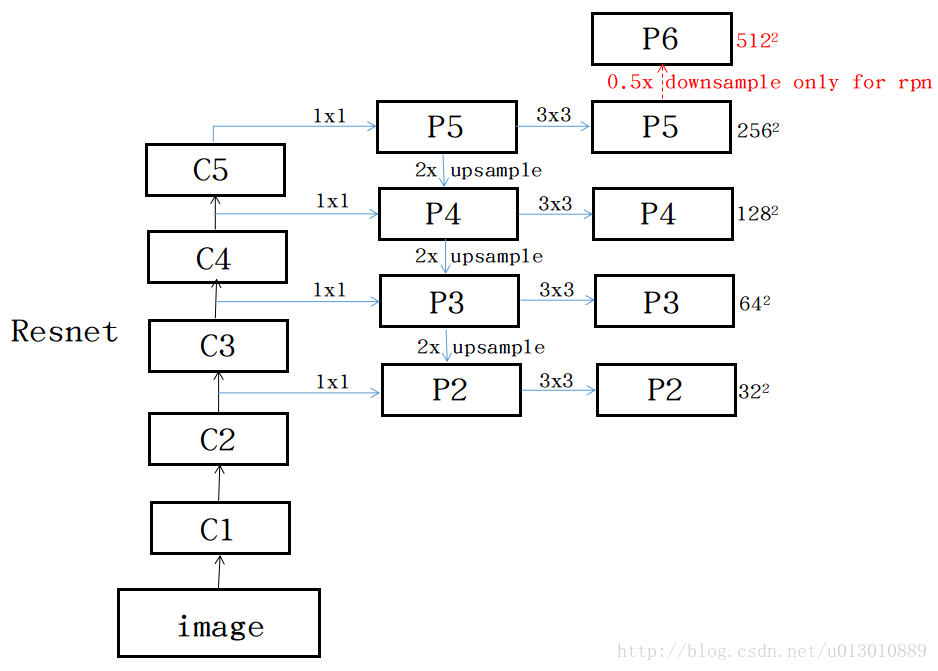
FPN的原理示意圖如下,上述包括一個自底向上的線路,一個自頂向下的線路,橫向連線(lateral connection),圖中放大的區域就是橫向連線。

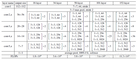
自底向上的路徑:自下而上的路徑是卷積網路的前饋計算,在前向過程中,feature map的大小在經過某些層後會改變,而在經過其他一些層的時候不會改變,作者將不改變feature map大小的層歸為一個stage,因此每次抽取的特徵都是每個stage的最後一個層輸出,這樣就能構成特徵金字塔。 具體而言,對於ResNets,通過這個表格我們可以知道,conv2,conv3,conv4和conv5就是一個stage,我們使用每個階段的最後一個residual block輸出的特徵啟用輸出。 對於conv2,conv3,conv4和conv5輸出,我們將這些最後residual block的輸出表示為{C2,C3,C4,C5},並且它們相對於輸入影象具有{4, 8, 16, 32} 的步長(也就是相對於輸入的影象縮小了4,8,16,32倍)。
自頂向下的路徑:自頂向下的路徑通過對在空間上更抽象但語義更強高層特徵圖進行上取樣來幻化高解析度的特徵。也就是將低解析度的特徵圖做2倍上取樣(為了簡單起見,使用最近鄰上取樣)。橫向連線是將上取樣的結果和自底向上生成的相同大小的feature map進行融合。這個過程是迭代的,直到生成最終的解析度圖。
也就是說:
(1)down-top就是每個residual block(C1去掉了,太大太耗記憶體了),scale縮小2,C2,C3,C4,C5(1/4, 1/8, 1/16, 1/32)。
(2)top-down就是把高層的低分辨強語義的feature 最近鄰上取樣2x
(3)lateral conn 就是把C2通過1x1卷積,使其的channel和top-down過來的一樣
具體的流程如下:
(1)利用256個1*1的卷積核對C5進行卷積,生成解析度最低但語義最強的feature P5,開始迭代 。
(2)然後P5上取樣放大2倍,C4經過一個1*1*256的卷積後與放大後P5尺寸相加,也就是融合。
經過上述兩個步驟問為什麼是256個卷積核,由於金字塔的所有層次都像傳統的特徵化影象金字塔一樣使用共享分類器/迴歸器,因此我們在所有特徵圖中固定特徵維度(通道數,記為d)。我們在本文中設定d = 256,因此所有額外的卷積層都有256
(3)以此迭代下去到P2結束
(4)對於生成的每一個Pk,後面還加一個3*3的卷積(原文說reduce the aliasing effect of upsampling) ,其目的是消除上取樣的混疊效應(aliasing effect)。
(5)最終生成的feature map結果是P2,P3,P4,P5,和原來自底向上的卷積結果C2,C3,C4,C5一一對應。
另外還將FPN用在了RPN中,原來的RPN網路是以主網路的某個卷積層輸出的feature map作為輸入,簡單講就是隻用這一個尺度的feature map。但是現在要將FPN嵌在RPN網路中,生成不同尺度特徵並融合作為RPN網路的輸入。在每一個scale層,都定義了不同大小的anchor,對於P2,P3,P4,P5,P6這些層,定義anchor的大小為32^2,64^2,128^2,256^2,512^2,另外每個scale層都有3個長寬對比度:1:2,1:1,2:1。所以整個特徵金字塔有15種anchor。
對上述的理解總的來說可以用下面這一張圖概括。
還有一個問題,RPN生成roi後對應feature時在哪個level上取呢?
k0是faster rcnn時在哪取feature map呢?例如resnet那篇文章是在C4取的,k0=4(C5相當於fc,也有在C5取的,在後面再多新增fc),比如roi是w/2,h/2,那麼k=k0-1=4-1=3 。這裡224是ImageNet的標準輸入。

還有個問題,從不同level取feature做roipooling後需要分類和迴歸,這些各個level需要共享嗎?本文的做法是共享,還有一點不同的是resnet論文中是把C5作為fc來用的,本文由於C5已經用到前面feature了,所以採用在後面加fc6 fc7,注意這樣是比把C5弄到後面快一點。
2.detectron中的引數
理解了原理,看這些引數就容易多了
# --------------------------------------------------------------------------- #
# FPN 引數
# --------------------------------------------------------------------------- #
__C.FPN = AttrDict()

#是否開啟FPN,True:開啟 FPN
__C.FPN.FPN_ON = False

# FPN 特徵層的通道維度Channel dimension
__C.FPN.DIM = 256

# True,初始化側向連線lateral connections 輸出 0
__C.FPN.ZERO_INIT_LATERAL = False

# 最粗糙coarsest FPN 層的步長
# 用於將輸入正確地補零,是需要的
__C.FPN.COARSEST_STRIDE = 32

#
# FPN 可以只是 RPN、或只是目標檢測,或兩者都用.
#

# True, 採用 FPN 用於目標檢測 RoI 變換
__C.FPN.MULTILEVEL_ROIS = False
# RoI-to-FPN 層的對映啟發式 超引數
__C.FPN.ROI_CANONICAL_SCALE = 224  # s0:相當於最後公式裡的原圖大小224
__C.FPN.ROI_CANONICAL_LEVEL = 4  # k0: where s0 maps to,相當於在C4取
# FPN 金字塔pyramid 的最粗糙層Coarsest level,即P5
__C.FPN.ROI_MAX_LEVEL = 5
# FPN 金字塔pyramid 的最精細層Finest level,即P2
__C.FPN.ROI_MIN_LEVEL = 2

# True,在 RPN 中使用 FPN
__C.FPN.MULTILEVEL_RPN = False
# FPN 金字塔pyramid應用於FPN的最粗糙層Coarsest level,即P6
__C.FPN.RPN_MAX_LEVEL = 6
# FPN 金字塔pyramid應用於FPN的最精細層Finest level,即P2
__C.FPN.RPN_MIN_LEVEL = 2
# FPN RPN anchor 長寬比aspect ratios
__C.FPN.RPN_ASPECT_RATIOS = (0.5, 1, 2)
# 在 RPN_MIN_LEVEL 上 RPN anchors 開始的尺寸
# RPN anchors start at this size on RPN_MIN_LEVEL
# The anchor size doubled each level after that
# With a default of 32 and levels 2 to 6, we get anchor sizes of 32 to 512
__C.FPN.RPN_ANCHOR_START_SIZE = 32  #如果檢測小物體可以適當調小
# 使用額外的 FPN 層levels, as done in the RetinaNet paper
__C.FPN.EXTRA_CONV_LEVELS = False
3.detectron中的程式碼
def add_fpn(model, fpn_level_info):
    """Add FPN connections based on the model described in the FPN paper."""
    # FPN levels are built starting from the highest/coarest level of the
    # backbone (usually "conv5"). First we build down, recursively constructing
    # lower/finer resolution FPN levels. Then we build up, constructing levels
    # that are even higher/coarser than the starting level.
    """
    FPN levels 是從骨幹backbone 網路的 highest/coarest level(通常為 conv5) 開始構建的.
    首先向下,遞迴地(recursively)構建 lower/finer 解析度的 FPN levels(P5,P4,P3,...);
    然後向上,構建比起始 level higher/coarser 解析度的 FPN levels(P6).
    """
    fpn_dim = cfg.FPN.DIM
    min_level, max_level = get_min_max_levels()
    # Count the number of backbone stages that we will generate FPN levels for
    # starting from the coarest backbone stage (usually the "conv5"-like level)
    # E.g., if the backbone level info defines stages 4 stages: "conv5",
    # "conv4", ... "conv2" and min_level=2, then we end up with 4 - (2 - 2) = 4
    # backbone stages to add FPN to.
    num_backbone_stages = (
        len(fpn_level_info.blobs) - (min_level - LOWEST_BACKBONE_LVL)
    )

    #這裡將conv2_x到conv5_x的輸出都稱為lateral_input_blobs,可以稱為橫向連結的輸入
    lateral_input_blobs = fpn_level_info.blobs[:num_backbone_stages]
    output_blobs = [
        'fpn_inner_{}'.format(s)
        for s in fpn_level_info.blobs[:num_backbone_stages]
    ]
    fpn_dim_lateral = fpn_level_info.dims  #(2048,1024,512,256)
    xavier_fill = ('XavierFill', {})

    # For the coarsest backbone level: 1x1 conv only seeds recursion
    if cfg.FPN.USE_GN:
        # use GroupNorm
        c = model.ConvGN(
            lateral_input_blobs[0],
            output_blobs[0],  # note: this is a prefix
            dim_in=fpn_dim_lateral[0],
            dim_out=fpn_dim,
            group_gn=get_group_gn(fpn_dim),
            kernel=1,
            pad=0,
            stride=1,
            weight_init=xavier_fill,
            bias_init=const_fill(0.0)
        )
        output_blobs[0] = c  # rename it
    else: #首先對conv5_x的輸出進行卷積,卷積的大小為1×1×256,得到P5
        model.Conv(
            lateral_input_blobs[0],  #輸入層:res5_2_sum
            output_blobs[0],         #輸出層:fpn_inner_res5_2_sum
            dim_in=fpn_dim_lateral[0], #輸入的特徵圖的大小:2048
            dim_out=fpn_dim,       #中間卷積核個數:256
            kernel=1,   #卷積核的大小
            pad=0,
            stride=1,
            weight_init=xavier_fill,
            bias_init=const_fill(0.0)
        )

    #
    # Step 1: recursively build down starting from the coarsest backbone level
    #  從 coarest backbone level 開始,遞迴地向下構建 FPN levels

    # For other levels add top-down and lateral connections
    for i in range(num_backbone_stages - 1):
        add_topdown_lateral_module(
            model,
            output_blobs[i],             # top-down blob   P5,fpn_inner_res5_2_sum
            lateral_input_blobs[i + 1],  # lateral blob    P5上取樣後要與conv4的輸出橫向連結,res4_5_sum
            output_blobs[i + 1],         # next output blob   將P5上取樣後的與conv4橫向連結,得到的結果為fpn_inner_res4_5_sum,也就是P4啦
            fpn_dim,                     # output dimension    256
            fpn_dim_lateral[i + 1]       # lateral input dimension  橫向連結的輸入的大小,也就是conv4的輸入的大小,1024
        )

    # Post-hoc scale-specific 3x3 convs
    blobs_fpn = []
    spatial_scales = []
    for i in range(num_backbone_stages):
        if cfg.FPN.USE_GN:
            # use GroupNorm
            fpn_blob = model.ConvGN(
                output_blobs[i],
                'fpn_{}'.format(fpn_level_info.blobs[i]),
                dim_in=fpn_dim,
                dim_out=fpn_dim,
                group_gn=get_group_gn(fpn_dim),
                kernel=3,
                pad=1,
                stride=1,
                weight_init=xavier_fill,
                bias_init=const_fill(0.0)
            )
        else: #對於每一個Pk,增加3*3的卷積
            fpn_blob = model.Conv(
                output_blobs[i],
                'fpn_{}'.format(fpn_level_info.blobs[i]),
                dim_in=fpn_dim,  #輸入:256
                dim_out=fpn_dim, #輸出:256
                kernel=3,
                pad=1,
                stride=1,
                weight_init=xavier_fill,
                bias_init=const_fill(0.0)
            )
        blobs_fpn += [fpn_blob]  #這個blobs_fpn是最終的FPN每一層的
        spatial_scales += [fpn_level_info.spatial_scales[i]]

    #
    # Step 2: build up starting from the coarsest backbone level
    #

    # Check if we need the P6 feature map
    if not cfg.FPN.EXTRA_CONV_LEVELS and max_level == HIGHEST_BACKBONE_LVL + 1:
        # Original FPN P6 level implementation from our CVPR'17 FPN paper
        P6_blob_in = blobs_fpn[0] #P6的輸入是P5的輸出 gpu_0/fpn_res5_2_sum
        P6_name = P6_blob_in + '_subsampled_2x'  #gpu_0/fpn_res5_2_sum_subsampled_2x
        # Use max pooling to simulate stride 2 subsampling
        P6_blob = model.MaxPool(P6_blob_in, P6_name, kernel=1, pad=0, stride=2)   #gpu_0/fpn_res5_2_sum_subsampled_2x
        blobs_fpn.insert(0, P6_blob)   #增加P6_blob
        spatial_scales.insert(0, spatial_scales[0] * 0.5)

    # Coarser FPN levels introduced for RetinaNet
    if cfg.FPN.EXTRA_CONV_LEVELS and max_level > HIGHEST_BACKBONE_LVL:
        fpn_blob = fpn_level_info.blobs[0]
        dim_in = fpn_level_info.dims[0]
        for i in range(HIGHEST_BACKBONE_LVL + 1, max_level + 1):
            fpn_blob_in = fpn_blob
            if i > HIGHEST_BACKBONE_LVL + 1:
                fpn_blob_in = model.Relu(fpn_blob, fpn_blob + '_relu')
            fpn_blob = model.Conv(
                fpn_blob_in,
                'fpn_' + str(i),
                dim_in=dim_in,
                dim_out=fpn_dim,
                kernel=3,
                pad=1,
                stride=2,
                weight_init=xavier_fill,
                bias_init=const_fill(0.0)
            )
            dim_in = fpn_dim
            blobs_fpn.insert(0, fpn_blob)
            spatial_scales.insert(0, spatial_scales[0] * 0.5)

    return blobs_fpn, fpn_dim, spatial_scales
最終生成的結構為:
| P6 | gpu_0/fpn_res5_2_sum_subsampled_2x |
| P5 | gpu_0/fpn_res5_2_sum |
| P4 | gpu_0/fpn_res4_5_sum |
| P3 | gpu_0/fpn_res3_3_sum |
| P2 | gpu_0/fpn_res2_2_sum |