Opencv影象處理---基於距離變換和分水嶺演算法的影象分割
阿新 • • 發佈:2018-12-16
程式碼
#include <opencv2/opencv.hpp>
#include <iostream>
using namespace std;
using namespace cv;
int main(int, char** argv)
{
    // Load the image
    Mat src = imread(argv[1]);
    // Check if everything was fine
    if (!src.data)
        return -1;
    // Show source image
    imshow("Source Image", src);
    // Change the background from white to black, since that will help later to extract
    // better results during the use of Distance Transform
    for( int x = 0; x < src.rows; x++ ) {
      for( int y = 0; y < src.cols; y++ ) {
          if ( src.at<Vec3b>(x, y) == Vec3b(255,255,255) ) {
            src.at<Vec3b>(x, y)[0] = 0;
            src.at<Vec3b>(x, y)[1] = 0;
            src.at<Vec3b>(x, y)[2] = 0;
          }
        }
    }
    // Show output image
    imshow("Black Background Image", src);
    // Create a kernel that we will use for accuting/sharpening our image
    Mat kernel = (Mat_<float>(3,3) <<
            1,  1, 1,
            1, -8, 1,
            1,  1, 1); // an approximation of second derivative, a quite strong kernel
    // do the laplacian filtering as it is
    // well, we need to convert everything in something more deeper then CV_8U
    // because the kernel has some negative values,
    // and we can expect in general to have a Laplacian image with negative values
    // BUT a 8bits unsigned int (the one we are working with) can contain values from 0 to 255
    // so the possible negative number will be truncated
    Mat imgLaplacian;
    Mat sharp = src; // copy source image to another temporary one
    filter2D(sharp, imgLaplacian, CV_32F, kernel);
    src.convertTo(sharp, CV_32F);
    Mat imgResult = sharp - imgLaplacian;
    // convert back to 8bits gray scale
    imgResult.convertTo(imgResult, CV_8UC3);
    imgLaplacian.convertTo(imgLaplacian, CV_8UC3);
    // imshow( "Laplace Filtered Image", imgLaplacian );
    imshow( "New Sharped Image", imgResult );
    src = imgResult; // copy back
    // Create binary image from source image
    Mat bw;
    cvtColor(src, bw, CV_BGR2GRAY);
    threshold(bw, bw, 40, 255, CV_THRESH_BINARY | CV_THRESH_OTSU);
    imshow("Binary Image", bw);
    // Perform the distance transform algorithm
    Mat dist;
    distanceTransform(bw, dist, CV_DIST_L2, 3);
    // Normalize the distance image for range = {0.0, 1.0}
    // so we can visualize and threshold it
    normalize(dist, dist, 0, 1., NORM_MINMAX);
    imshow("Distance Transform Image", dist);
    // Threshold to obtain the peaks
    // This will be the markers for the foreground objects
    threshold(dist, dist, .4, 1., CV_THRESH_BINARY);
    // Dilate a bit the dist image
    Mat kernel1 = Mat::ones(3, 3, CV_8UC1);
    dilate(dist, dist, kernel1);
    imshow("Peaks", dist);
    // Create the CV_8U version of the distance image
    // It is needed for findContours()
    Mat dist_8u;
    dist.convertTo(dist_8u, CV_8U);
    // Find total markers
    vector<vector<Point> > contours;
    findContours(dist_8u, contours, CV_RETR_EXTERNAL, CV_CHAIN_APPROX_SIMPLE);
    // Create the marker image for the watershed algorithm
    Mat markers = Mat::zeros(dist.size(), CV_32SC1);
    // Draw the foreground markers
    for (size_t i = 0; i < contours.size(); i++)
        drawContours(markers, contours, static_cast<int>(i), Scalar::all(static_cast<int>(i)+1), -1);
    // Draw the background marker
    circle(markers, Point(5,5), 3, CV_RGB(255,255,255), -1);
    imshow("Markers", markers*10000);
    // Perform the watershed algorithm
    watershed(src, markers);
    Mat mark = Mat::zeros(markers.size(), CV_8UC1);
    markers.convertTo(mark, CV_8UC1);
    bitwise_not(mark, mark);
//    imshow("Markers_v2", mark); // uncomment this if you want to see how the mark
                                  // image looks like at that point
    // Generate random colors
    vector<Vec3b> colors;
    for (size_t i = 0; i < contours.size(); i++)
    {
        int b = theRNG().uniform(0, 255);
        int g = theRNG().uniform(0, 255);
        int r = theRNG().uniform(0, 255);
        colors.push_back(Vec3b((uchar)b, (uchar)g, (uchar)r));
    }
    // Create the result image
    Mat dst = Mat::zeros(markers.size(), CV_8UC3);
    // Fill labeled objects with random colors
    for (int i = 0; i < markers.rows; i++)
    {
        for (int j = 0; j < markers.cols; j++)
        {
            int index = markers.at<int>(i,j);
            if (index > 0 && index <= static_cast<int>(contours.size()))
                dst.at<Vec3b>(i,j) = colors[index-1];
            else
                dst.at<Vec3b>(i,j) = Vec3b(0,0,0);
        }
    }
    // Visualize the final image
    imshow("Final Result", dst);
    waitKey(0);
    return 0;
}
解釋與結果
- 載入源影象並檢查它是否載入沒有任何問題,然後顯示它:
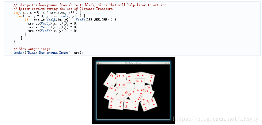
- 如果我們有一個白色背景影象,最好將其轉換為黑色。 當我們應用距離變換時,這將有助於我們更容易區分前景物件:
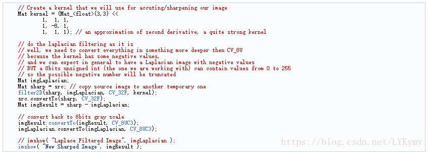
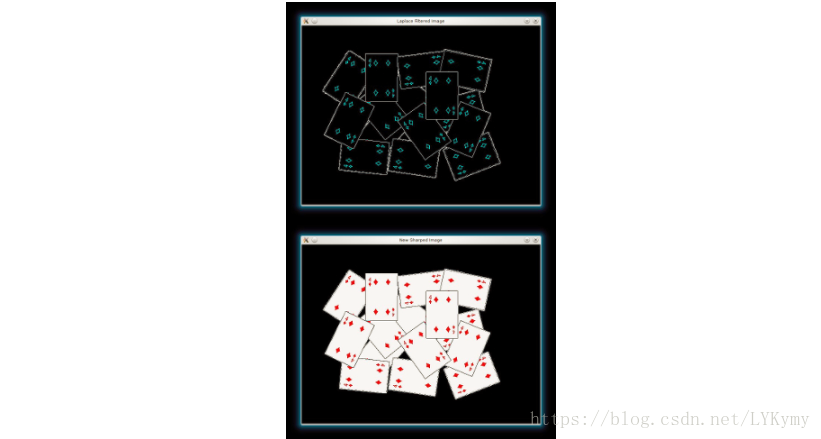
- 我們將銳化我們的影象,以銳化前景物件的邊緣。 我們將應用具有相當強濾波器的拉普拉斯濾波器(近似二階導數):
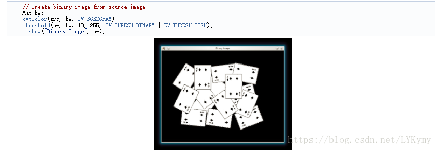
- 現在我們將新的銳化源影象分別轉換為灰度和二進位制:
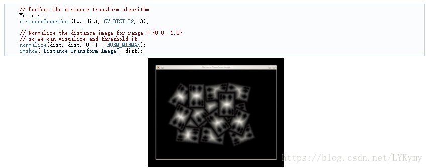
- 我們現在準備在二進位制影象上應用距離變換。 此外,我們對輸出影象進行標準化,以便能夠對結果進行視覺化和閾值處理:
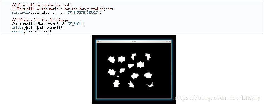
- 我們對dist影象進行閾值處理,然後執行一些形態學操作(即擴張),以便從上面的影象中提取峰值:
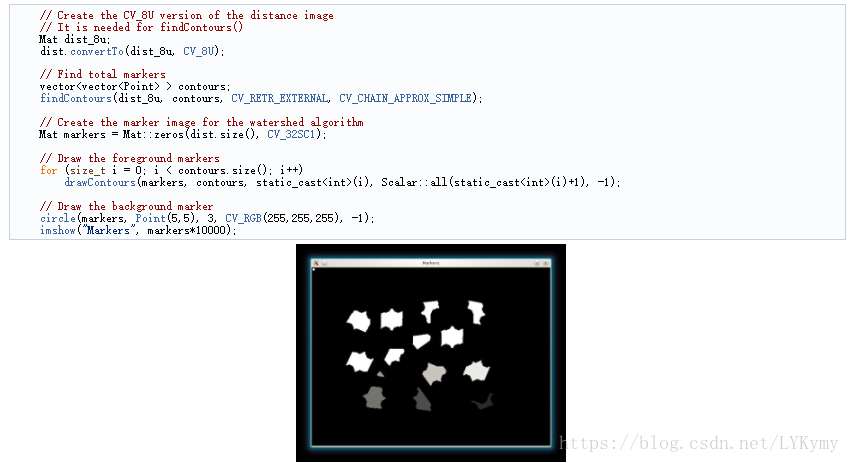
- 我們在cv :: findContours函式的幫助下為分水嶺演算法建立種子/標記:
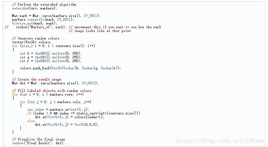
- 最後,我們可以應用分水嶺演算法,並可視化結果: