Lets revisit the basic anatomy of an index:

Default index in postgres is of type BTree which constitutes a BTree or a balanced tree of index entries and index leaf nodes which store physical address of an index entry

An index lookup requires three steps:

1. Tree traversal
2. Following the leaf node chain
3. Fetching the table data

The above steps are explained in detail here.

Tree traversal is the only step that has an upper bound for the number of accessed blocks — the index depth. The other two steps might need to access many blocks — their upper bound can be as large as the full table scan.

An Index Scan performs a B-tree traversal, walks through the leaf nodes to find all matching entries, and fetches the corresponding table data. It is like an INDEX RANGE SCAN followed by a TABLE ACCESS BY INDEX ROWID operation.Following the leaf node chain requires getting ROW ID’s that fulfill the customer_id

condition: in our case, it has max limit of 200 row ID’s. Since these index leaf nodes are stored in a sorted manner, their access is upper bounded by the length of this chain or total rows in the table. The next step is the TABLE ACCESS BY INDEX ROWID operation. It uses the ROWID from previous step to fetch the rows — all columns — from the table. Here the db engine must fetch the rows individually hitting each record in page and bringing them in memory for retrieval. It involves random access IO’s apart from read operations. We decided it might be worthwhile to look at how these query result rows were distributed on physical memory. In postgres, location of a row is given by ctidwhich is a tuple . ctid is of type tid (tuple identifier), called ItemPointer in the C code. Per documentation:

This is the data type of the system column ctid. A tuple ID is a pair (block number, tuple index within block) that identifies the physical location of the row within its table.

The distribution was like this:

customer_id | product_id | ctid — — — — — — -+ — — — — — —  1254 | 284670 | (3789,28) 1254 | 18934 | (7071,73) 1254 | 14795 | (8033,19) 1254 | 10908 | (9591,60) 1254 | 95032 | (11017,83) 1254 | 318562 | (11134,65) 1254 | 18854 | (11275,54) 1254 | 109943 | (11827,76) 1254 | 105 | (16309,104) 1254 | 3896 | (18432,8) 1254 | 3890 | (20062,90) 1254 | 318550 | (20488,84) 1254 | 37261 | (20585,62) ...

Clearly, rows for a particular customer id were far from each other on disk. This seemed to explain the high execution times of queries having customer_id in WHERE clause. The db engine was hitting pages on disk for retrieving each row. There was high random access IO. What if we could bring all rows of a particular customer together? If done, the engine might be able to retrieve all rows in result set in one go.

Postgres provides a CLUSTER command which physically rearranges the rows on disk based on a given column. But given constraints like acquiring a READ WRITE lock on table and requiring 2.5x the table size made it tricky to use. We began to explore if we could write the table in customer id rows sorted manner. The application which was writing these rows was a Spark application using collaborative filtering algorithm to derive recommended products.

Part II This required us to dig deeper into how Spark writes to Postgres. It writes data partition wise. Now, what is this partition?

Spark being a distributed computing framework distributes a particular data frame into partitions amongst its workers. It allows you to explicitly partition a dataframe based on a partition key to ensure minimal shuffling (bring partitions from one worker to another for reading/writing operations). Looking at the code we found that we had partitioned on product_id for a particular transformation operation.

This meant that the data written to our postgres table should be product_id wise, i.e. that is rows of all customer ID’s whose recommendations were a particular product ID should be clubbed together . We tested our hypothesis by looking at results of :

SELECT *, ctid FROM personalized_recommendations WHERE product_id = 284670 product_id | customer_id |   ctid------------+-------------+----------     284670 |        1133 | (479502,71)     284670 |        2488 | (479502,72)     284670 |        3657 | (479502,73)     284670 |        2923 | (479502,74)     284670 |        6911 | (479502,75)     284670 |        9018 | (479502,76)     284670 |        4263 | (479502,77)     284670 |        1331 | (479502,78)     284670 |        3242 | (479502,79)     284670 |        3661 | (479502,80)     284670 |        9867 | (479502,81)     284670 |        7066 | (479502,82)     284670 |       10267 | (479502,83)     284670 |        7499 | (479502,84)     284670 |        8011 | (479502,85)

Yes indeed, all rows of a particular product ID were together on the table. So if we instead partitioned on customer_id , our objective of bringing all result rows of a customer_id would be met. This post here talks about repartition in detail.We repartitioned the df by:

df.repartition($”customer_id”)

And wrote the final df to postgres. Now we checked for distribution of rows.

dse_db=> SELECT product_id,customer_id,ctid FROM personalized_recommendations WHERE customer_id = 28460limit 20; product_id | customer_id | ctid — — — — — — + — — — — — — -+ — — — — —  28460 | 1133 | (0,24) 28460 | 2488 | (4,7) 28460 | 3657 | (9,83) 28460 | 2923 | (18,54) 28460 | 6911 | (20,42) 28460 | 9018 | (31,59) 28460 | 4263 | (35,79) 28460 | 1331 | (38,14) 28460 | 3242 | (40,41) 28460 | 3661 | (55,105) 28460 | 9867 | (57,21) 28460 | 7066 | (61,28) 28460 | 10267 | (62,63) 28460 | 7499 | (66,8)

Alas, the table is still not pivoted on customer_id . What did we do wrong?

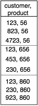
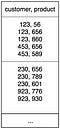
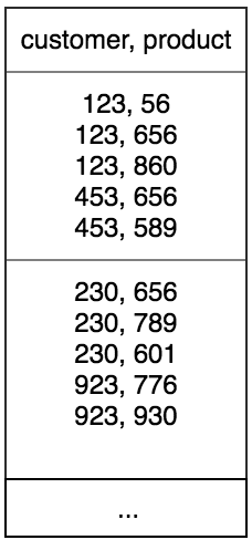
Apparently, the default number of partitions on which data is rearranged is 200. But since the number of distinct customer ID’s were greater than 200 (~1 crore) , this meant that a single partition will contain recommended products of more that 1 customer as seen in the figure below. In this case, close to (~1 crore/200=50,000) customers.

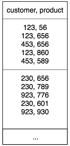
When this particular partition will be written to the db, this will still not ensure that all rows belonging to a customer_id be written together. We then sorted rows within a partition by customer_id:

df.repartition($”customer_id”).sortWithinPartitions($”customer_id”)

It is an expensive operation for spark to perform but nevertheless necessary for us. We did this and wrote again to the database. Next we checked for distribution.

customer_id | product_id | ctid — — — — — — -+ — — — — — — + — — — — — - 1254 | 284670 | (212,95) 1254 | 18854 | (212,96) 1254 | 18850 | (212,97) 1254 | 318560 | (212,98) 1254 | 318562 | (212,99) 1254 | 318561 | (212,100) 1254 | 10732 | (212,101) 1254 | 108 | (212,102) 1254 | 11237 | (212,103) 1254 | 318058 | (212,104) 1254 | 38282 | (212,105) 1254 | 3884 | (212,106) 1254 | 31 | (212,107) 1254 | 318609 | (215,1) 1254 | 2 | (215,2) 1254 | 240846 | (215,3) 1254 | 197964 | (215,4) 1254 | 232970 | (215,5) 1254 | 124472 | (215,6) 1254 | 19481 | (215,7) …

Voila! Its now pivoted on customer_id (tears of joy :,-) ). The final test still remains. Will the query execution now be faster. Lets see what the query planner says.

EXPLAIN ANALYZE SELECT * FROM personalized_recommendations WHERE customer_id = 25001;

QUERY PLAN 

Bitmap Heap Scan on personalized_recommendations(cost=66.87..13129.94 rows=3394 width=38) (actual time=2.843..3.259 rows=201 loops=1) Recheck Cond: (customer_id = 25001) Heap Blocks: exact=2 -> Bitmap Index Scan on personalized_recommendations_temp_customer_id_idx (cost=0.00..66.02 rows=3394 width=0) (actual time=1.995..1.995 rows=201 loops=1) Index Cond: (customer_id = 25001) Planning time: 0.067 ms Execution time: 3.322 ms

Execution time came down from ~100 ms to ~3ms.

This optimization really helped us use personalized recommendations to serve a variety of use cases like generating targeted advertising pushes for a growing consumer base of more than 1lakh users in bulk etc. When this was first launched, size of the data was ~12 GB. Now in the past 1 year, it has grown to ~22GB but rearranging the records in the table has helped to keep database retrieval latencies to minimal. Although now, the time taken for Spark application to generate these recommendations, arranging the dataframe and writing to database has increased manifold. But since that happens in batch mode, it is still acceptable. As the data grows and the use cases to serve it, there will be many more challenges to solve.