
How Do I Predict Time Series?
How Do I Predict Time Series?
Forecasting, modelling and predicting time series is increasingly becoming popular in a number of fields. Time series prediction is all about forecasting future. Every second a large quantity of data is stored in servers across the world. This data is invaluable and can help us predict future.
Forecasting time series is not always a straight forward process. There are number of techniques to build models that can estimate and forecast future time points. Subsequently, these models can help us make calculated decisions which in return can reduce risk and increase return. Additionally, building reliable and robust forecasting models are essential when predicting behaviors of market movements.
Please read FinTechExplained disclaimer before proceeding.
It is crucial for us to understand how time series works so that we can accurately predict future.
What Is Covered In This Article?
Forecasting future accurately requires deep understanding of current state of our target variables. My aim is to build the required knowledge in this article. It covers basics of time series.
In particular, it provides:
- Explanation of what time series is
- What covariance stationary time series means
- How we characterize cycles and seasonality in time series
- Lastly, I will explain ARIMA, in particular GARCH and EWMA models
What Is Time Series?
Time series is a number of observations collected over a successive period of time. To emphasize, if we observe a variable for a set of time points and record its behaviour then the variable will form a trend against time. This trend is known as time series.
- Variable — anything that changes over time
- Time periods — Can be daily, weekly, monthly, yearly etc
- Variable Behaviour — Quantifiable value
Time Series Examples
There are a large number of time series examples, including:
- Daily exchange rates or stock price movements
- Yearly population of a country over 50 years
- Weekly weight change in pounds of a person for a year
- Yearly GDP of a country for 50 years
- Number of cars manufactured in a car factory semi-annually
- Rate of interest rate change over time


Time series analysis is complex in nature. This is mainly due to the analysis required to discover hidden factors and noise.
Occasionally models are too simplistic and it is not always apparent to account for the factors that have inner relationships between each other.
Past Is Important
Most time series data is dependent on its past values. Recent past values are good indicators of a variable’s behaviour. Lagged values of a variable such as an exchange rate are regressed over one or more lagged values of itself to predict the current and future values of a variable. Missing data is often filled with past data. It can also be calculated from past data such as by taking average.
Interrelationships of data are then calculated. These relationships are then formulated into models which are used to forecast future time points. Occasionally, weighted sum of present and past values are used to forecast future values.
Role Of Lag Operator
When dealing with past data to forecast future data, it is important to understand that a lag operator is used. Lag operator enables models to quantify how past, present and future values are linked to each other. Lag operators use finite order polynomials and are essential tool to model a time series.


For example, let’s assume we are recording London’s daily temperature and want to build a model that forecasts temperature. There is higher probability that the temperature tomorrow will be similar to what it is today. It is unlikely to snow tomorrow if it is melting hot today.
Also assume we are recording world’s population on yearly basis. We notice that each year the population increases by 1%. It is unlikely for the rate of growth of population to increase by 100% next year. This is the fundamental concept of forecasting time series data.
Past can be used to predict future. Some time series data is totally random.
Past data can be a good indicator of future data
Current value of most of the variables e.g. interest rate depend on their past values. Financial series such as stock prices, income of a company etc. usually exhibit exponential growth/decay. They can be modeled using regression analysis technique:
Y(at Time T) = Intercept x Exponential ^(rate of growth at time T)
- Y: What we want to predict
- Intercept: If we plot the data where x-axis is time and y-axis are the actual values of Y then intercept is the value when time is 0.
From the observed data, a trend can be seen by plotting the data.
Linear Vs Non-Linear Time Series
Once we plot a variable’s value against time on a scatter plot, we can observe the shape of the graph to determine if it is linear or non-linear. In simplistic terms, linear time series trends are straight lines where as non-linear time series trends have curves.
Linear trends are easier to forecast and they provide better bit for the data. Non linear trends can be exponential, and at times quadratic. Linear functions have a constant gradient, known as rate of growth/decay. Negative gradient indicates negative correlation and positive gradient indicates positive relationship between time and values of the variable.
Non Linear Time Series To Linear Time Series
Non linear time series can also be converted from non-linear to log-linear series by taking a log on each side:
ln(Y at time T) = ln(Intercept) x Rate of growth at time T
Then log of Y can be plotted against time axis.


Deterministic Vs Non-Deterministic Time Series
Time series can be deterministic or non-deterministic in nature. Deterministic time series always behave in an expected manner where as non-deterministic time series is stochastic or random in nature.
Once time series is observed, a range of metrics can be calculated to understand its behaviour. These metrics include expected value (mean), variance, covariance, correlation to name a few.
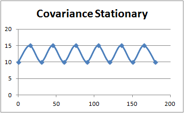
Covariance Stationary Time Series
To be able to forecast a time series model, it is important to ensure that it is covariance stationary.
If a time series mean, variance and covariance with past and future values do not change over time then the model is known to be covariance stationary.
Benefits Of Covariance Stationary Models
Covariance stationary time series models are reliable and better estimate the data. If a model is not covariance stationary then it makes the process of predicting trends difficult which then makes forecasting near to impossible. Thus we consider such models as unstable.
To achieve better forecast, time series needs to be covariance stationary. This implies that the time series does not hold any hidden relationships between different time points and the behaviour is stable.
For example if we wanted to measure house sales for a year in an area and we build a model that depends on employment and inflation rate to forecast house prices then we need to ensure that the two chosen factors are independent i.e. employment and inflation rates are not correlated with each other. Additionally we need to ensure that the lagged time points are not correlated with each other. Lastly, mean and variance is constant. Otherwise we will end up building an unreliable model.
Wold’s representation theorem evaluates covariance stationary as a prerequisite for time series modelling. White noise is a process where time series process has a zero mean, constant variance and no serial correlation between data points.
Assume we observed a series of exchange rates over 180 days and plotted the exchange rates over time. Once plotted, we notice that the mean and spread of curves do not change with time and there is no obvious up or downward moving trend. Thus such a time series is likely to be a stationary time series.

3 Criteria Of Time Series Covariance Stationary
Time series needs to meet following three criteria to be stationary:
1. Constant Mean
Mean or expected value of a time series over successive time periods needs to be constant for a time series to be considered covariance stationary. This implies that the expected value should not be time dependent.
How do I check if expected value (mean) is changing in a time series?
To check if mean of a time series is constant, divide the time series into equal sets (potentially 2 sets) and calculate expected value of each set by summing all values of time series and then dividing the calculated total by the total number of values.
- The calculated mean of each set should be constant.
How does a changing mean time series look?
If mean of a time series is time dependent then an increasing trend is experienced in a time series as shown below:

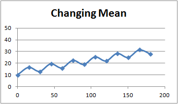
We can see that the value of exchange rate is dependent on time.
2. Constant Variance
Variance or standard deviation of a time series needs to be constant over time and should not be dependent on time. This is the second criteria for a time series to be covariance stationary.
Note: Standard Deviation Is The Square Root Of Variance
How do I check if variance is changing in a time series?
To check if variance is changing, divide the time series into equal sets (potentially 2 sets) and calculate expected value for each set by summing all values within a set and then dividing the calculated sum by the total number of values in a set. Variance is then calculated by first taking difference between each value and the mean and lastly summing differences and then dividing the total of differences by the total number of values in the set. Repeat the calculation for all of the required sets and check if the variance value for all sets is constant.
How does a changing variance time series look?
The change in spread and height of each trend indicates changing variance as shown below


Spread is changing with time and variance is time dependent
3. Constant Covariance
To understand covariance, it’s important to comprehend correlation.
Correlation measures strength of the relationship between variables co-movement. It is the standardised variance of two assets. Correlation is always between -1 and 1. Value of -1 indicates that the variables are negatively correlated and +1 shows that the variables are positively correlated. 0 indicates that there is no correlation amongst the target variables.
Covariance is calculated by multiplying Correlation of assets to the Standard Deviation of assets.
Covariance(X,Y) At Time Point T = Expected Value of (X, Y) — ((Expected Value of X) x (Expected Value of Y) for each time point T. X, Y are the two target variables.
How do I check if covariance is changing in a time series?
To check if covariance is changing, calculate the covariance value for two successive points in your time series and check that it is not time dependent. Therefore covariance is calculated from current and lagged time points.
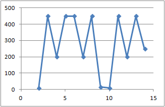
How does changing covariance time series look?
If a covariance is not constant in a time series then the time series exhibits randomness. Additionally, time series distribution changes without any obvious pattern. This indicates that the time series time points have changing correlation. This behaviour is also known as hetroscedasticity.

Dickey-Fuller Test can also be used to determine if time series is stationary. More on hypothesis analysis is covered in my blog “Hypothesis Analysis Explained”.
Seasonality
Once we plot time series data on a scatter plot and if we observe re-occurring patterns then it indicates existence of seasonality effects. Seasonality effects can be due to specific calendar days such as holidays. For example, if we are observing shopping center sales over a period of time then it is likely to experience an increase in sales during holidays.
To further explain, let’s assume we want to forecast our house gas bill for next year. We collect monthly gas bill for past 4 years and plot it as a line chart. We are likely to notice an increase in gas bill during winter. This pattern is a classic example of seasonality effect as shown below


If Trend Exists => Time Series Is Not Stationary
How Do We Eliminate Seasonality?
Sometimes it is not suitable to adjust time series for seasonality, particularly when it is important to capture all trends and changes in time series. However if the sole aim of the analysis is to only measure non-seasonal variations in a time series then the time series can be seasonally adjusted. It can take a number of forms, from interpolating values to reduce seasonality, to taking average of points, to completely excluding seasonality.
Two of the most common methodologies include:
- Differencing — Seasonality adjusted time series
- If time series is non stationary then differencing can be applied to observations to eliminate seasonality. A common methodology is to find observed values for time points when seasonality is experienced and then remove difference due seasonality. As an example, if we were forecasting interest rate and experienced a constant increase in interest rate point every Monday then we can find the interest rate value for last Monday and subtract it from the current value of Monday to eliminate seasonality effect.
2. Regression analysis with seasonal dummy variables:
- A number of variables are introduced to represent specific slots in the time. For example, if we are capturing stock price changes on daily basis and if every Friday, we experience large movements in market then Fridays can be represented as the seasonal dummy variable. Dummy variables take a value of 0 to 1, where 0 implies ignoring effect of Friday. It is as if we are telling the model to forget about seasonal dummy variables.
- Seasonal dummy variables can be used to account for specific holidays. It is important to carefully consider the seasonal dummy variables.
Finally
It is crucial to understand time series analysis as it is used in nearly all fields; from finance to artificial intelligence to data science. This article covered basics of time series along with an explanation of covariance stationary time series and seasonality. ARIMA models can be used to forecast time series which I have explained in the article.
Hope it helps.