Implement Back Propagation in Neural Networks

When building neural networks, there are several steps to take. Perhaps the two most important steps are implementing forward and backward propagation. Both these terms sound really heavy and are always scary to beginners. The absolute truth is that these techniques can be properly understood if they are broken down into their individual steps. In this tutorial, we will focus on backpropagation and the intuition behind every step of it.

What is Back Propagation?

This is simply a technique in implementing neural networks that allow us to calculate the gradient of parameters in order to perform gradient descent and minimize our cost function. Numerous scholars have described back propagation as arguably the most mathematically intensive part of a neural network. Relax though, as we will completely decipher every part of back propagation in this tutorial.

Implementing Back Propagation

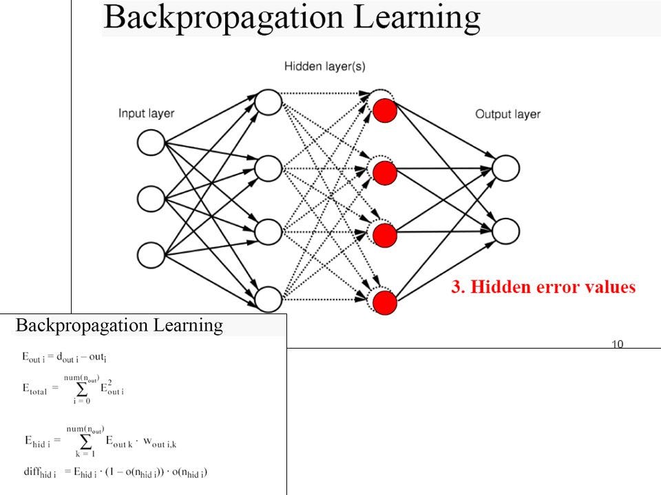
Assuming a simple two-layer neural network — one hidden layer and one output layer. We can perform back propagation as follows

Initialize the weight and bias to be used for the neural network: This involves randomly initializing the weights and biases of the neural networks. The gradient of these parameters will be obtained from the backward propagation and used to update gradient descent.

#Import Numpy libraryimport numpy as np#set seed for reproducability np.random.seed(100)

#We will first initialize the weights and bias needed and store them in a dictionary called W_Bdef initialize(num_f, num_h, num_out):        '''    Description: This function randomly initializes the weights and biases of each layer of the neural network        Input Arguments:    num_f - number of training features    num_h -the number of nodes in the hidden layers    num_out - the number of nodes in the output         Output:         W_B - A dictionary of the initialized parameters.        '''        #randomly initialize weights and biases, and proceed to store in a dictionary    W_B = {        'W1': np.random.randn(num_h, num_f),        'b1': np.zeros((num_h, 1)),        'W2': np.random.randn(num_out, num_h),        'b2': np.zeros((num_out, 1))    }    return W_B

Perform forward propagation: This involves calculating both the linear and activation outputs for both the hidden layer and the output layer.

For the hidden layer:

We will be using the relu activation function as seen below:

#We will now proceed to create functions for each of our activation functionsdef relu (Z):        '''    Description: This function performs the relu activation function on a given number or matrix.         Input Arguments:    Z - matrix or integer        Output:        relu_Z -  matrix or integer with relu performed on it        '''    relu_Z = np.maximum(Z,0)        return relu_Z

For the Output layer:

We will be using the sigmoid activation function as seen below:

def sigmoid (Z):        '''    Description: This function performs the sigmoid activation function on a given number or matrix.         Input Arguments:    Z - matrix or integer        Output:        sigmoid_Z -  matrix or integer with sigmoid performed on it        '''    sigmoid_Z = 1 / (1 + (np.exp(-Z)))        return sigmoid_Z

Perform the forward propagation:

#We will now proceed to perform forward propagationdef forward_propagation(X, W_B):        '''    Description: This function performs the forward propagation in a vectorized form         Input Arguments:    X - input training examples    W_B - initialized weights and biases        Output:        forward_results - A dictionary containing the linear and activation outputs        '''        #Calculate the linear Z for the hidden layer    Z1 = np.dot(X, W_B['W1'].T)  + W_B['b1']        #Calculate the activation ouput for the hidden layer    A = relu(Z1)        #Calculate the linear Z for the output layer    Z2 = np.dot(A, W_B['W2'].T) + W_B['b2']        #Calculate the activation ouput for the ouptu layer    Y_pred = sigmoid(Z2)         #Save all ina dictionary     forward_results = {"Z1": Z1,                      "A": A,                      "Z2": Z2,                      "Y_pred": Y_pred}        return forward_results

Perform Backward Propagation: Calculate the gradients of the cost relative to the parameters relevant for gradient descent. In this case, dLdZ2, dLdW2, dLdb2, dLdZ1, dLdW1 and dLdb1. These parameters will be combined with the learning rate to perform gradient descent. We will implement a vectorized version of the backpropagation for a number of training samples — no_examples.

The step by step guide is as follows:

• Obtain Results from forwarding propagation as seen below:

forward_results = forward_propagation(X, W_B)Z1 = forward_results['Z1']A = forward_results['A']Z2 = forward_results['Z2']Y_pred = forward_results['Y_pred']

• Obtain the number of training samples as seen below:

no_examples = X.shape[1]

• Calculate the Loss of the function:

L = (1/no_examples) * np.sum(-Y_true * np.log(Y_pred) - (1 - Y_true) * np.log(1 - Y_pred))

• Calculate the gradient for each parameter as seen below:

dLdZ2= Y_pred - Y_truedLdW2 = (1/no_examples) * np.dot(dLdZ2, A.T)dLdb2 = (1/no_examples) * np.sum(dLdZ2, axis=1, keepdims=True)dLdZ1 = np.multiply(np.dot(W_B['W2'].T, dLdZ2), (1 - np.power(A, 2)))dLdW1 = (1/no_examples) * np.dot(dLdZ1, X.T)dLdb1 = (1/no_examples) * np.sum(dLdZ1, axis=1, keepdims=True)

• Store the calculated gradients needed for gradient descent in a dictionary:

gradients = {"dLdW1": dLdW1,             "dLdb1": dLdb1,             "dLdW2": dLdW2,             "dLdb2": dLdb2}

• Return the loss and the stored gradients:

return gradients, L

Here is the complete backward propagation function:

def backward_propagation(X, W_B, Y_true):    '''Description: This function performs the backward propagation in a vectorized form         Input Arguments:    X - input training examples    W_B - initialized weights and biases    Y_True - the true target values of the training examples        Output:         gradients - the calculated gradients of each parameter    L - the loss function        '''        # Obtain the forward results from the forward propagation         forward_results = forward_propagation(X, W_B)    Z1 = forward_results['Z1']    A = forward_results['A']    Z2 = forward_results['Z2']    Y_pred = forward_results['Y_pred']        #Obtain the number of training samples        no_examples = X.shape[1]        # Calculate loss     L = (1/no_examples) * np.sum(-Y_true * np.log(Y_pred) - (1 - Y_true) * np.log(1 - Y_pred))        #Calculate the gradients of each parameter needed for gradient descent     dLdZ2= Y_pred - Y_true    dLdW2 = (1/no_examples) * np.dot(dLdZ2, A.T)    dLdb2 = (1/no_examples) * np.sum(dLdZ2, axis=1, keepdims=True)    dLdZ1 = np.multiply(np.dot(W_B['W2'].T, dLdZ2), (1 - np.power(A, 2)))    dLdW1 = (1/no_examples) * np.dot(dLdZ1, X.T)    dLdb1 = (1/no_examples) * np.sum(dLdZ1, axis=1, keepdims=True)        #Store gradients for gradient descent in a dictionary     gradients = {"dLdW1": dLdW1,             "dLdb1": dLdb1,             "dLdW2": dLdW2,             "dLdb2": dLdb2}        return gradients, L

Many people always think that back propagation is difficult, but as you have seen in this tutorial, it is not. Understanding every step is imperative to grasp the entire back-propagation technique. Also, it pays to have a good grasp of mathematics — linear algebra and calculus — in order to understand how the individual gradients of each function are calculated. With these tools, back propagation should be a piece of cake! In practice, back propagation is usually handled for you by the Deep Learning framework you are using. However, it pays to understand the inner workings of this technique as it can sometimes help you understand why your neural network may not be training well.

I will post more blogs in future about back propagation to get you depper understanding, so stay tuned:)