Cross-Correlation of Currency Pairs In R (ccf)
Cross-Correlation of Currency Pairs In R (ccf)
When working with a time series, one important thing we wish to determine is whether one series “causes” changes in another. In other words, is there a strong correlation between a time series and another given a number of lags? The way we can detect this is through measuring cross-correlation
For instance, one time series could serve as a lagging indicator. This is where the effect of a change in one time series transfers to the other time series several periods later. This is quite common in economic data; e.g. an economic shock having an effect on GDP two quarters later.
But how do we measure the lag where this is significant? One very handy way of doing so in R is using the ccf
Running this function allows us to determine the lag at which the correlation between two time series is strongest.
Two important things that we must ensure when we run a cross-correlation:
- Our time series is stationary.
- Once we have chosen the suitable lag, we are then able to detect and correct for serial correlation if necessary.
If you are unfamiliar with these, then please review two of my previous posts on stationarity and serial correlation:
Cross-Correlation Across Currency Pairs
We will use quantmod to download data for the currency pairs CAD/USD, CHF/USD, EUR/USD, and then examine the nature of cross-correlation between these different time series.
> library(quantmod) > #Quantmod> CADUSD<-getSymbols("DEXCAUS", src = "FRED")> CHFUSD<-getSymbols("DEXSZUS", src = "FRED")> EURUSD<-getSymbols("DEXUSEU", src = "FRED") > #Store within dataframes> cadusd=na.omit(data.frame(tail(log(DEXCAUS),100)))> chfusd=na.omit(data.frame(tail(log(DEXSZUS),100)))> eurusd=na.omit(data.frame(tail(log(DEXUSEU),100)))> attach(cadusd)> attach(chfusd)> attach(eurusd)
> plot(DEXCAUS,type='l')> plot(DEXSZUS,type='l')> plot(DEXUSEU,type='l')
As you can see from the above, we are downloading the past 100 days of data for the respective currency pairs, omitting any NA values, and log-transforming our time series.
Stationarity Testing
Let us now formally test for stationarity using the ADF and KPSS tests:
> library(tseries)> adf.test(cadusd$DEXCAUS)
Augmented Dickey-Fuller Test
data: cadusd$DEXCAUSDickey-Fuller = -1.424, Lag order = 4, p-value =0.8148alternative hypothesis: stationary
> adf.test(chfusd$DEXSZUS)
Augmented Dickey-Fuller Test
data: chfusd$DEXSZUSDickey-Fuller = -1.3124, Lag order = 4, p-value =0.861alternative hypothesis: stationary
> adf.test(eurusd$DEXUSEU)
Augmented Dickey-Fuller Test
data: eurusd$DEXUSEUDickey-Fuller = -2.2158, Lag order = 4, p-value =0.4873alternative hypothesis: stationary
> kpss.test(cadusd$DEXCAUS)
KPSS Test for Level Stationarity
data: cadusd$DEXCAUSKPSS Level = 1.2213, Truncation lag parameter = 2,p-value = 0.01
Warning message:In kpss.test(cadusd$DEXCAUS) : p-value smaller than printed p-value> kpss.test(chfusd$DEXSZUS)
KPSS Test for Level Stationarity
data: chfusd$DEXSZUSKPSS Level = 3.016, Truncation lag parameter = 2,p-value = 0.01
Warning message:In kpss.test(chfusd$DEXSZUS) : p-value smaller than printed p-value> kpss.test(eurusd$DEXUSEU)
KPSS Test for Level Stationarity
data: eurusd$DEXUSEUKPSS Level = 2.8434, Truncation lag parameter = 2,p-value = 0.01
Warning message:In kpss.test(eurusd$DEXUSEU) : p-value smaller than printed p-value
As we can see, the p-value for the ADF test is much higher than 0.05, indicating non-stationarity. Non-stationarity is also indicated by KPSS given that the p-values are lower than 0.05. In this regard, the plots still indicate a trend and the two series are therefore differenced:
> diffcadusd=diff(cadusd$DEXCAUS,1)> diffchfusd=diff(chfusd$DEXSZUS,1)> diffeurusd=diff(eurusd$DEXUSEU,1)
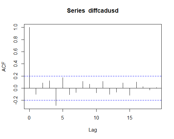
> acf(diffcadusd)

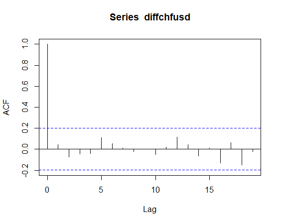
> acf(diffchfusd)

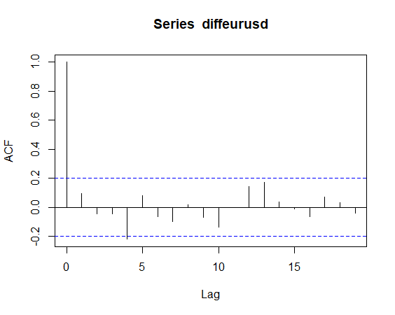
> acf(diffeurusd)

> adf.test(diffcadusd)
Augmented Dickey-Fuller Test
data: diffcadusdDickey-Fuller = -4.1964, Lag order = 4, p-value =0.01alternative hypothesis: stationary
Warning message:In adf.test(diffcadusd) : p-value smaller than printed p-value
> adf.test(diffchfusd)
Augmented Dickey-Fuller Test
data: diffchfusdDickey-Fuller = -3.8888, Lag order = 4, p-value =0.01766alternative hypothesis: stationary
> adf.test(diffeurusd)
Augmented Dickey-Fuller Test
data: diffeurusdDickey-Fuller = -4.5462, Lag order = 4, p-value =0.01alternative hypothesis: stationary
Warning message:In adf.test(diffeurusd) : p-value smaller than printed p-value
> kpss.test(diffcadusd)
KPSS Test for Level Stationarity
data: diffcadusdKPSS Level = 0.12321, Truncation lag parameter = 2,p-value = 0.1
Warning message:In kpss.test(diffcadusd) : p-value greater than printed p-value> kpss.test(diffchfusd)
KPSS Test for Level Stationarity
data: diffchfusdKPSS Level = 0.13076, Truncation lag parameter = 2,p-value = 0.1
Warning message:In kpss.test(diffchfusd) : p-value greater than printed p-value
> kpss.test(diffeurusd)
KPSS Test for Level Stationarity
data: diffeurusdKPSS Level = 0.086579, Truncation lag parameter =2, p-value = 0.1
Warning message:In kpss.test(diffeurusd) : p-value greater than printed p-value
We now see that the ADF test shows a p-value below 0.05, and the KPSS test now shows a p-value above 0.05. This indicates trend stationarity.
Moreover, when we plot the ACF for the two differenced variables, stationarity is indicated given that we see sudden drops in the acf after the first lag.
Cross-Correlation: Output and Plot
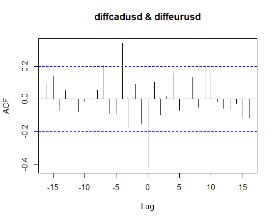
Let us now plot the cross-correlation (CCF function) for the three differenced currency pairs:
> ccf1<-ccf(diffcadusd,diffeurusd)> ccf1
Autocorrelations of series ‘X’, by lag
-16 -15 -14 -13 -12 -11 -10 -9 0.096 0.139 -0.069 0.050 -0.019 -0.077 -0.015 -0.002 -8 -7 -6 -5 -4 -3 -2 -1 0.053 0.206 -0.092 -0.094 0.339 -0.177 0.092 -0.153 0 1 2 3 4 5 6 7 -0.423 0.102 -0.095 0.014 0.160 -0.069 0.001 0.131 8 9 10 11 12 13 14 15 -0.051 0.204 0.153 -0.019 -0.057 -0.066 -0.026 -0.109 16 -0.117

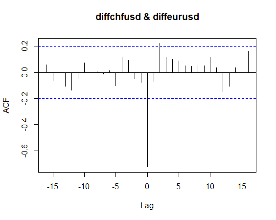
> ccf2<-ccf(diffchfusd,diffeurusd)> ccf2
Autocorrelations of series ‘X’, by lag
-16 -15 -14 -13 -12 -11 -10 -9 0.060 -0.061 0.000 -0.108 -0.135 -0.044 0.074 0.000 -8 -7 -6 -5 -4 -3 -2 -1 0.008 -0.013 0.016 -0.101 0.120 0.091 -0.051 -0.075 0 1 2 3 4 5 6 7 -0.727 -0.067 0.223 0.115 0.098 0.088 0.053 0.048 8 9 10 11 12 13 14 15 0.051 0.050 0.116 0.035 -0.146 -0.107 0.038 0.060 16 0.163

> ccf3<-ccf(diffcadusd,diffchfusd)> ccf3
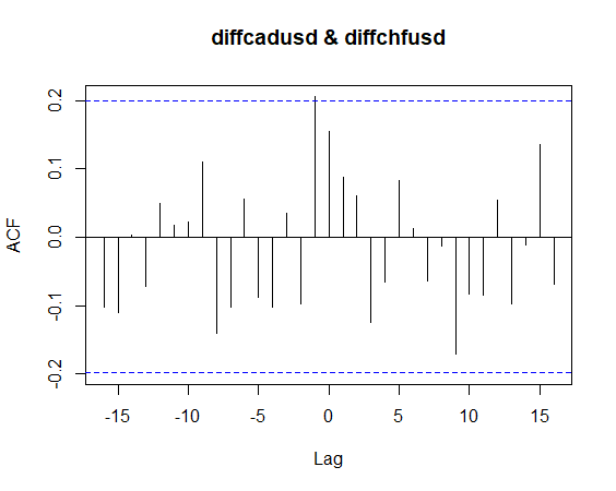
Autocorrelations of series ‘X’, by lag
-16 -15 -14 -13 -12 -11 -10 -9 -0.102 -0.111 0.003 -0.072 0.050 0.017 0.023 0.110 -8 -7 -6 -5 -4 -3 -2 -1 -0.141 -0.102 0.055 -0.088 -0.103 0.034 -0.097 0.206 0 1 2 3 4 5 6 7 0.156 0.089 0.061 -0.125 -0.066 0.083 0.013 -0.064 8 9 10 11 12 13 14 15 -0.013 -0.171 -0.083 -0.085 0.054 -0.097 -0.012 0.136 16 -0.068

Observations
Examining our cross-correlation plots yields some interesting results.
- We see that there is a strong negative correlation at lag 0 for both the CAD/USD — EUR/USD and CHF/USD — EUR/USD.
- For the CAD/USD — CHF/USD pair, the strongest correlation occurs at time (t-1), indicating that Granger Causality may exist between these pairs. i.e. a movement in the CAD/USD at time t-1 may have an effect on the CHF/USD at time t.
- In the case of the first two autocorrelations, we see that while the strongest is at lag 0, there are other autocorrelations that occur throughout the series at different lags.
Conclusion
In this tutorial, you have learned:
- What is a cross-correlation
- How to test a time series for stationarity
- How to convert a non-stationary series into a stationary one
- Generate a cross-correlation using ccf
Many thanks for reading, and if you are interested in learning how we can run the above analysis in Python, please feel free to read my follow-up article here.
