1. Read the dataframe

I will import and name my dataframe df, in Python this will be just two lines of code. This will work if you saved your train.csv in the same folder where your notebook is.

import pandas as pddf = pd.read_csv('train.csv')

Scala will require more typing.

var df = sqlContext    .read    .format("csv")    .option("header", "true")    .option("inferSchema", "true")    .load("Filestore/tables/train.csv")

Let’s see what’s going on up here. Scala does not assume your dataset has a header, so we need to specify that. Also, Python will assign automatically a dtype to the dataframe columns, while Scala doesn’t do so, unless we specify .option("inferSchema", "true"). Also notice that I did not import Spark Dataframe, because I practice Scala in

Notice: booleans are capitalized in Python, while they are all lower-case in Scala!

2. Display the first rows of the dataframe

In Python, df.head() will show the first five rows by default: the output will look like this.

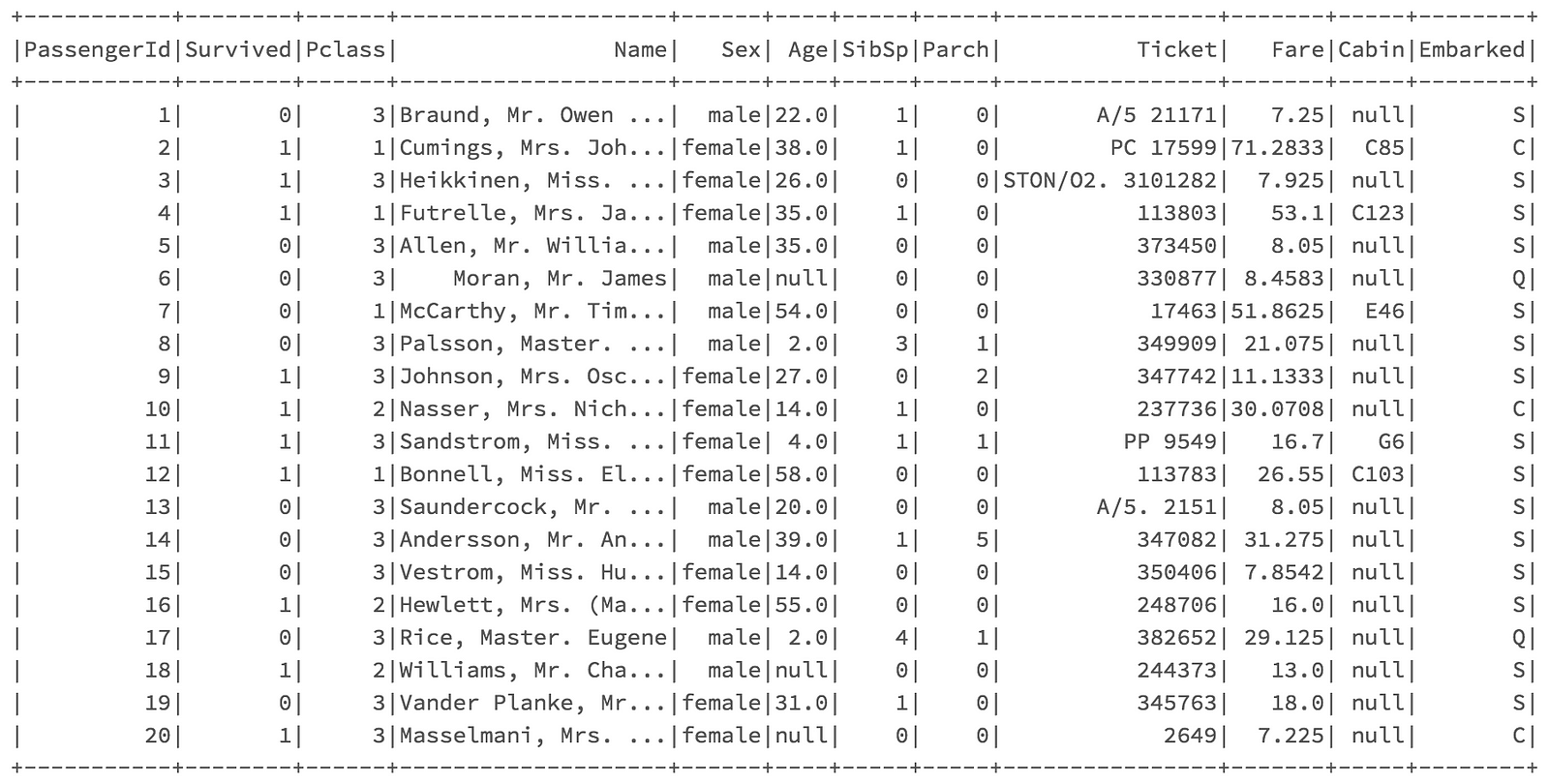
If you want to see a number of rows different than five, you can just pass a different number in the parenthesis. Scala, with its df.show(),will display the first 20 rows by default.

If we want to keep it shorter, and also get rid of the ellipsis in order to read the entire content of the columns, we can run df.show(5, false).

3. Dataframe Columns and Dtypes

To retrieve the column names, in both cases we can just type df.columns: Scala and Pandas will return an Array and an Index of strings, respectively.

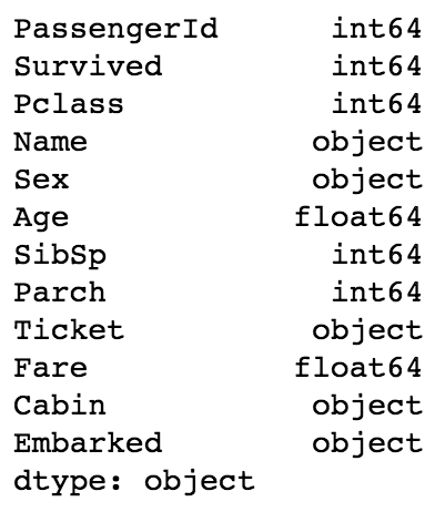
If we want to check the dtypes, the command is again the same for both languages: df.dtypes. Pandas will return a Series object, while Scala will return an Array of tuples, each tuple containing respectively the name of the

column and the dtype. So, if we are in Python and we want to check what type is the Age column, we run df.dtypes['Age'], while in Scala we will need to filter and use the Tuple indexing: df.dtypes.filter(colTup => colTup._1 == "Age").

4. Summary Statistics

This is another thing that every Data Scientist does while exploring his/her data: summary statistics. For every numerical column, we can see information such as count, mean, median, deviation, so on and so forth, to see immediately if there is something that doesn’t look right. In both cases this will return a dataframe, where the columns are the numerical columns of the original dataframe, and the rows are the statistical values.

In Python, we type df.describe(), while in Scala df.describe().show(). The reason we have to add the .show() in the latter case, is because Scala doesn’t output the resulting dataframe automatically, while Python does so (as long as we don’t assign it to a new variable).

5. Select Columns

Suppose we want to see a subset of columns, for example Name and Survived.

In Python we can use either df[['Name','Survived]] or df.loc[:,['Name','Survived] indistinctly. Remember that the : in this case means “all the rows”.

In Scala, we will type df.select("Name","Survived").show(). If you want to assign the subset to a new variable, remember to omit the .show().

6. Filtering

Let’s say we want to have a look at the Name and Pclass of the passengers who survived. We will need to filter a condition on the Survived column and then select the the other ones.

In Python, we will use .loc again, by passing the filter in the rows place and then selecting the columns with a list. Basically like the example above but substituting the : with a filter, which means df.loc[df['Survived'] == 1, ['Name','Pclass']].

In Scala we will use .filter followed by .select, which will be df.filter("Survived = 1").select("Name","Pclass").show().

6.1. Filtering null values

If we want to check the null values, for example in the Embarked column, it will work like a normal filter, just with a different condition.

In Python, we apply the .isnull() when passing the condition, in this casedf[df['Embarked'].isnull()]. Since we didn’t specify any columns, this will return a dataframe will all the original columns, but only the rows where the Embarked values are empty.

In Scala, we will use .filter again: df.filter("Embarked IS NULL").show(). Notice that the boolean filters we pass in Scala, kind of look like SQL queries.

7. Imputing Null Values

We should always give some thought before imputing null values in a dataset, because it is something that will influence our final model and we want to be careful with that. However, just for demonstrative purposes, let’s say we want to impute the string “N/A” to the null values in our dataframe.

We can do so in Python with either df = df.fillna('N/A') or df.fillna('N/A', inplace = True).

In Scala, quite similarly, this would be achieved with df = df.na.fill("N/A"). Remember to not use the .show() in this case, because we are assigning the revised dataframe to a variable.

8. Renaming Columns

This is something that you will need to for sure in Scala, since the machine learning models will need two columns named features and label in order to be trained. However, this is something you might want to do also in Pandas if you don’t like how a column has been named, for example. For this purpose, we want to change the Survived column into label.

In Python we will pass a dictionary, where the key and the value are respectively the old and the new name of the column. In this case, it will be df.rename(columns = {"Survived": "label"}, inplace = True).

In Scala, this equals to df = df.withColumnRenamed("Survived", "label").

9. Group By and Aggregation

Let’s say we want to calculate the maximum Age for men and women distinctively, in this case .groubpby comes in handy. Not only to retrieve the maximum value; after .groupby we can use all sorts of aggregation functions: mean, count, median, so on and so forth. We stick with .max() for this example.

In Python this will be df.groupby('Sex').mean()['Age']. If we don’t specify ['Age'] after .mean(), this will return a dataframe with the maximum values for all numerical columns, grouped by Sex.

In Scala, we will need to import the aggregation function we want to use, first.

import org.apache.spark.sql.functions.maxdf.groupBy("Sex").agg(max("Age")).show()

10. Create a New Column

This is really useful for feature engineering, we might want to combine two variables to see how their interaction is related to the target. For purely demonstrative purpose, let’s see how to create a column containing the product between Age and Fare.

In Python it is pretty straightforward.

df['Age_times_Fare'] = df['Age'] * df['Fare']

In Scala, we will need to put $ before the names of the columns we want to use, so that the column object with the corresponding name will be considered.

df = df.withColumn("AgeTimesFare", $"Age" * $"Fare")

11. Correlation

Exploring correlation among numerical variables and target is always convenient, and obtaining a matrix of correlation coefficients among all numeric variables is pretty easy in Python, just by running df.corr(). If you want to look at the correlation, let’s say between Age and Fare, we will just need to specify the columns: df[['Age','Fare']].corr().

In Scala, we will need to import first, and then run the command by specifying the columns.

import org.apache.spark.sql.functions.corrdf.select(corr("Age","Fare")).show()