A breath of fresh air with Decision Trees

A very versatile decision support tool, capable of fitting complex algorithms, that can perform both classification and regression tasks, and even multioutput tasks.

Trees are very interesting beings… they can start from a single branch and develop into a very complex network of branches with millions of leaves at their ends. It’s curious that a great number of technologies and methodologies are created based on what we see in Nature. Machine Learning Decision Tree algorithm is one of those cases!

A decision tree is a Supervised Machine Learning algorithm. This non-parametric system, contrary to Linear Regression models (which assume linearity), makes no underlying assumptions about the distribution of the errors or the data. It is a flowchart-like structure, composed of several questions (node) and depending on the answers (branch) given it will lead to a class label or value (leaf) when applied to any observation.

“Decision tree learning uses a decision tree (as a predictive model) to go from observations about an item (represented in the branches) to conclusions about the item’s target value (represented in the leaves). “— Wikipedia

Today’s post is about Classification and Regression Trees (CART). Scikit-Learn

Learning about CART by example : Iris Dataset

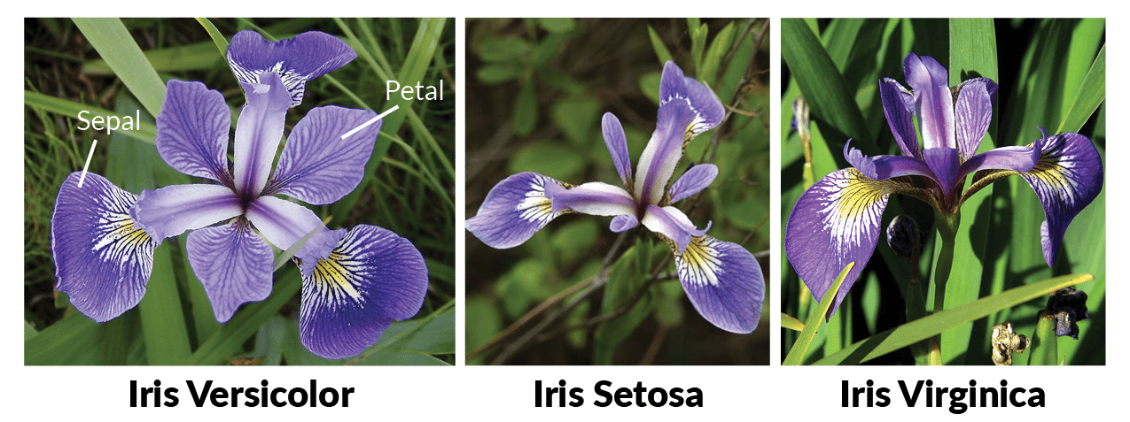
“The Iris flower dataset or Fisher’s Iris dataset is a multivariate dataset introduced by the British statistician and biologist Ronald Fisher in his 1936 paper ‘The use of multiple measurements in taxonomic problems as an example of linear discriminant analysis’.” — Wikipedia

This is one of the most used datasets for the typical “Hello World” in Data Science. The Iris Dataset contains four features (length and width of sepals and petals) of 50 samples of three species of Iris (Iris setosa, Iris virginica and Iris versicolor). Let’s use these measures to create a Decision Tree model to classify the species.

You can get the link to the full Python code of this example at the end of this article.

# Common importsimport numpy as npimport os

#to make this notebook's output stable across runsnp.random.seed(42)

# To plot pretty figures%matplotlib inlineimport matplotlibimport matplotlib.pyplot as plt

from sklearn.datasets import load_irisfrom sklearn.tree import DecisionTreeClassifier

iris = load_iris()X = iris.data[:,2:] #petal length and widthy = iris.target

tre_clf = DecisionTreeClassifier(max_depth = 2)tre_clf.fit(X,y)

SkLearn has a cool feature which allows us to visualise the generated Decision Tree by using the method export_graphviz() :

from sklearn.tree import export_graphviz

export_graphviz( tree_clf, out_file=”iris_tree.dot”, feature_names=iris.feature_names[2:], class_names=iris.target_names, rounded=True, filled=True )

Using the software graphviz you can convert this .dot file into a variety of format such as .PDF or .PNG.

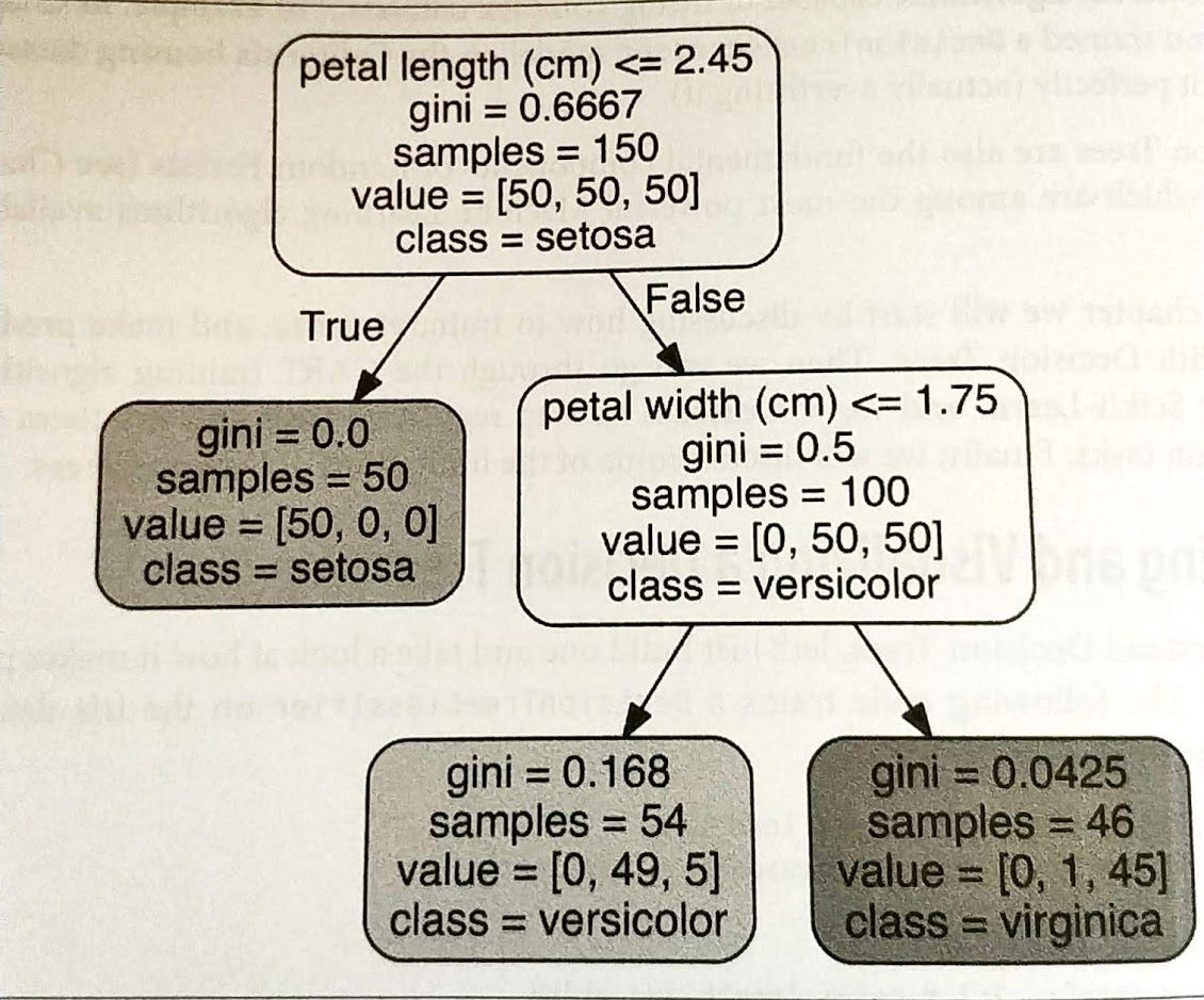
As you can see, this decision tree, in opposite to real life trees, has its root at the top. The first line of each internal node represents the condition. Based on this condition, the node splits into two other branches/edges. In the end, when a branch does not split anymore it is known as decision/leaf. Since our algorithm will have to classify our training data samples into the categories [setosa, versicolor, virginica] this a Classification Decision Tree.

Remember we are only considering two features to label our data, petal width and petal length.

“Scikit-Learn uses the CART algorithm, which produces only binary trees: nonleaf nodes always have two children (i.e. questions only have yes/no answers)”

Having our Decision Tree algorithm defined we can start to make some predictions. Let’s pick a random flower from our dataset. We start at the root node (depth 0). We see here that the feature chosen is “Petal Length” and our condition for splitting:

“Is the flower’s petal length smaller or equal to 2.45 cm?”

If we answer True then we move down to the respective child node (depth 1, left). Since, for this node there are no more branches we’ve reached the leaf. In this node, no questions are asked and the classed is attributed to our flower. Now, let’s consider another flower but this time the petal length is bigger than 2.45 cm. We now go to the node in depth 1 which assumes the feature “Petal Width” and the splitting condition to be:

“Is the flower’s petal width smaller or equal to 1.75 cm?”

As you can observe, this node has branches attached which means it has children nodes. According to our answer, we have to go further one more level in depth so to classify our flower. Independently of the given answer, we’ve reached our leaves and there are no more splitting conditions to approve. It seems like our system has reached the stopping point and is now able to label the flower.

Nodes attributes:

• Sample : counts how many training instances it applies to. It started at the root node (depth 0) with 150 observations. From that point, it divides according to the classification given.
• Value : how many training instances of each class this node applies to. For example, the last leaf on the right applies to 0 Iris-Setosa, 1 Iris-Versicolor and 45 Iris-Virginica.
• Gini : measures its impurity. A node is pure if all training instances it applies to belong to the same class.

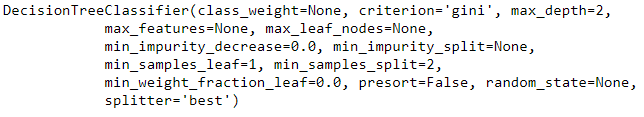
Now, that we’ve understood the theory behind CART let’s see it in action using Python’s library Scikit-Learn.

from matplotlib.colors import ListedColormap

def plot_decision_boundary(clf, X, y, axes=[0, 7.5, 0, 3], iris=True, legend=False, plot_training=True):

 x1s = np.linspace(axes[0], axes[1], 100) x2s = np.linspace(axes[2], axes[3], 100) x1, x2 = np.meshgrid(x1s, x2s) X_new = np.c_[x1.ravel(), x2.ravel()] y_pred = clf.predict(X_new).reshape(x1.shape)

 custom_cmap = ListedColormap([‘#fafab0’,’#9898ff’,’#a0faa0']) plt.contourf(x1, x2, y_pred, alpha=0.3, cmap=custom_cmap) if not iris: custom_cmap2 = ListedColormap([‘#7d7d58’,’#4c4c7f’,’#507d50']) plt.contour(x1, x2, y_pred, cmap=custom_cmap2, alpha=0.8) if plot_training: plt.plot(X[:, 0][y==0], X[:, 1][y==0], “yo”, label=”Iris-Setosa”) plt.plot(X[:, 0][y==1], X[:, 1][y==1], “bs”, label=”Iris-Versicolor”) plt.plot(X[:, 0][y==2], X[:, 1][y==2], “g^”, label=”Iris-Virginica”) plt.axis(axes)

 if iris: plt.xlabel(“Petal length”, fontsize=14) plt.ylabel(“Petal width”, fontsize=14)

 else: plt.xlabel(r”$x_1$”, fontsize=18) plt.ylabel(r”$x_2$”, fontsize=18, rotation=0) if legend: plt.legend(loc=”lower right”, fontsize=14)

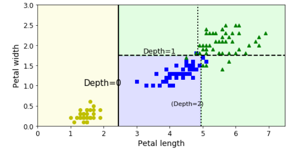
plt.figure(figsize=(8, 4))plot_decision_boundary(tree_clf, X, y)plt.plot([2.45, 2.45], [0, 3], “k-”, linewidth=2)plt.plot([2.45, 7.5], [1.75, 1.75], “k — “, linewidth=2)plt.plot([4.95, 4.95], [0, 1.75], “k:”, linewidth=2)plt.plot([4.85, 4.85], [1.75, 3], “k:”, linewidth=2)plt.text(1.40, 1.0, “Depth=0”, fontsize=15)plt.text(3.2, 1.80, “Depth=1”, fontsize=13)plt.text(4.05, 0.5, “(Depth=2)”, fontsize=11)

plt.show()

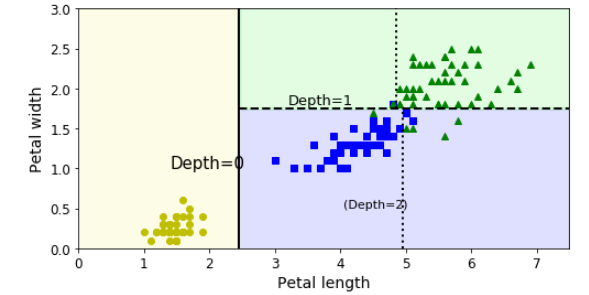
This is our algorithm’s decision boundaries. The thick vertical line represents the decision boundary for depth level 0, where the node is pure. Due to being a pure node, it cannot be split further hence the algorithm goes on to analysing and splitting the unpure area on the right where the petal width is equal to 1.75 cm (dashed line). Remember that in the beginning we set the stop splitting condition (number of depth level) equal to 2 (tree_clf = DecisionTreeClassifier(max_depth = 2)), which means our algorithm stops here.

Maximum depth refers to the the length of the longest path from a root to a leaf.

This would be the result if max_depth = 3.

If we intended to increase the algorithm’s performance we could increase it by pruning. For that, we would have to remove the branches that make use of features with low importance. Therefore, we would reduce the tree’s complexity and increase its prediction capacity by reducing the overfitting.