
CNN提取圖片特徵,之後用SVM分類
https://blog.csdn.net/qq_27756361/article/details/80479278
先用CNN提取特徵,之後用SVM分類,平臺是TensorFlow 1.3.0-rc0,python3.6
這個是我的一個小小的測試,下面這個連結是我主要參考的,在實現過程中,本來想使用vgg16或者VGG19做遷移來提取特徵,但是擔心自己的算力不夠,還有就是UCI手寫資料集本來就是一個不大的資料集,使用vgg16或vgg19有點殺雞用牛刀的感覺。於是放棄做遷移。
我的程式碼主要是基於下面連結來的。參考連結點選開啟連結
這個程式碼主要是,通過一個CNN網路,在網路的第一個全連線層也就h_fc1得到的一個一維的256的一個特徵向量,將這個特徵向量作為的svm的輸入。主要的操作是在程式碼行的140-146. 同時代碼也實現了CNN的過程(讀一下程式碼就知道)。
如果你要是知道你的CNN的結構,然後就知道在全連線層輸出的其實就是一個特徵向量。直接用這個特徵向量簡單處理輸入到svm中就可以。
具體的參考論文和程式碼資料集等,百度網盤
CNN卷積層簡介
CNN,有兩個卷積(5*5)池化層(2*2的maxPooling),然後兩個全連線層h_fc1和h_fc2,我只使用第一個全連線層h_fc1就提取了特徵。
然後中間的啟用函式使用的是relu函式,同時為了防止過擬合使用了dropout的技巧。然後這個程式碼中其實是實現了完整的CNN的的預測的,損失使用交叉熵,優化器使用了AdamOptimizer。
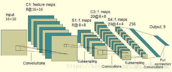
圖片大小的變化:
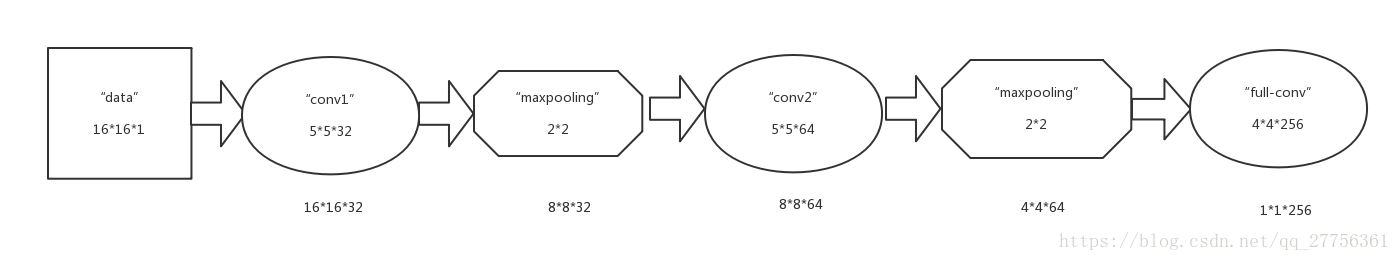
最後從全連線層提取的256維的向量。輸入svm。
SVM分類
SVM採用的是RBF核(高斯核),C取0.9
也可以嘗試線性核,我試了一下效果差不多,但是沒有高斯核分類效率好。
流程和實驗設計
流程:整理訓練網路的資料,對樣本進行處理 -> 建立卷積神經網路-> 將資料代入進行訓練 -> 儲存訓練好的模型(從全連線層提取特徵) -> 把資料代入模型獲得特徵向量 -> 用特徵向量代替原本的輸入送入SVM訓練 -> 測試時同樣將h_fc1轉換為特徵向量之後用SVM預測,獲得結果。
使用留出法樣本處理和評價:
1.將原樣本隨機地分為兩半。一份為訓練集,一份為測試集
2.重複1過程十次,得到十個訓練集和十個對應的測試集
3.取十份訓練集中的一份和其對應的測試集。代入到CNN和SVM中訓練。
4.依次取訓練集和測試集,則可完成十次第一步。
5.將十次的表現綜合評價,十次驗證取平均值,計算正確率、準確率、召回率、F1值。比如 F1 分數 , 用於測量不均衡資料的精度.
-
# coding=utf8 -
import random -
import numpy as np -
import tensorflow as tf -
from sklearn import svm -
from sklearn import preprocessing -
import time -
start = time.clock() -
right0 = 0.0 # 記錄預測為1且實際為1的結果數 -
error0 = 0 # 記錄預測為1但實際為0的結果數 -
right1 = 0.0 # 記錄預測為0且實際為0的結果數 -
error1 = 0 # 記錄預測為0但實際為1的結果數 -
for file_num in range(10): -
# 在十個隨機生成的不相干資料集上進行測試,將結果綜合 -
print('testing NO.%d dataset.......' % file_num) -
ff = open('digit_train_' + file_num.__str__() + '.data') -
rr = ff.readlines() -
x_test2 = [] -
y_test2 = [] -
-
for i in range(len(rr)): -
x_test2.append(list(map(int, map(float, rr[i].split(' ')[:256])))) -
y_test2.append(list(map(int, rr[i].split(' ')[256:266]))) -
ff.close() -
# 以上是讀出訓練資料 -
ff2 = open('digit_test_' + file_num.__str__() + '.data') -
rr2 = ff2.readlines() -
x_test3 = [] -
y_test3 = [] -
for i in range(len(rr2)): -
x_test3.append(list(map(int, map(float, rr2[i].split(' ')[:256])))) -
y_test3.append(list(map(int, rr2[i].split(' ')[256:266]))) -
ff2.close() -
# 以上是讀出測試資料 -
sess = tf.InteractiveSession() -
# 建立一個tensorflow的會話 -
# 初始化權值向量 -
def weight_variable(shape): -
initial = tf.truncated_normal(shape, stddev=0.1) -
return tf.Variable(initial) -
# 初始化偏置向量 -
def bias_variable(shape): -
initial = tf.constant(0.1, shape=shape) -
return tf.Variable(initial) -
# 二維卷積運算,步長為1,輸出大小不變 -
def conv2d(x, W): -
return tf.nn.conv2d(x, W, strides=[1, 1, 1, 1], padding='SAME') -
# 池化運算,將卷積特徵縮小為1/2 -
def max_pool_2x2(x): -
return tf.nn.max_pool(x, ksize=[1, 2, 2, 1], strides=[1, 2, 2, 1], padding='SAME') -
# 給x,y留出佔位符,以便未來填充資料 -
x = tf.placeholder("float", [None, 256]) -
y_ = tf.placeholder("float", [None, 10]) -
# 設定輸入層的W和b -
W = tf.Variable(tf.zeros([256, 10])) -
b = tf.Variable(tf.zeros([10])) -
# 計算輸出,採用的函式是softmax(輸入的時候是one hot編碼) -
y = tf.nn.softmax(tf.matmul(x, W) + b) -
# 第一個卷積層,5x5的卷積核,輸出向量是32維 -
w_conv1 = weight_variable([5, 5, 1, 32]) -
b_conv1 = bias_variable([32]) -
x_image = tf.reshape(x, [-1, 16, 16, 1]) -
# 圖片大小是16*16,,-1代表其他維數自適應 -
h_conv1 = tf.nn.relu(conv2d(x_image, w_conv1) + b_conv1) -
h_pool1 = max_pool_2x2(h_conv1) -
# 採用的最大池化,因為都是1和0,平均池化沒有什麼意義 -
# 第二層卷積層,輸入向量是32維,輸出64維,還是5x5的卷積核 -
w_conv2 = weight_variable([5, 5, 32, 64]) -
b_conv2 = bias_variable([64]) -
h_conv2 = tf.nn.relu(conv2d(h_pool1, w_conv2) + b_conv2) -
h_pool2 = max_pool_2x2(h_conv2) -
# 全連線層的w和b -
w_fc1 = weight_variable([4 * 4 * 64, 256]) -
b_fc1 = bias_variable([256]) -
# 此時輸出的維數是256維 -
h_pool2_flat = tf.reshape(h_pool2, [-1, 4 * 4 * 64]) -
h_fc1 = tf.nn.relu(tf.matmul(h_pool2_flat, w_fc1) + b_fc1) -
# h_fc1是提取出的256維特徵,很關鍵。後面就是用這個輸入到SVM中 -
# 設定dropout,否則很容易過擬合 -
keep_prob = tf.placeholder("float") -
h_fc1_drop = tf.nn.dropout(h_fc1, keep_prob) -
# 輸出層,在本實驗中只利用它的輸出反向訓練CNN,至於其具體數值我不關心 -
w_fc2 = weight_variable([256, 10]) -
b_fc2 = bias_variable([10]) -
y_conv = tf.nn.softmax(tf.matmul(h_fc1_drop, w_fc2) + b_fc2) -
cross_entropy = -tf.reduce_sum(y_ * tf.log(y_conv)) -
# 設定誤差代價以交叉熵的形式 -
train_step = tf.train.AdamOptimizer(1e-4).minimize(cross_entropy) -
# 用adma的優化演算法優化目標函式 -
correct_prediction = tf.equal(tf.argmax(y_conv, 1), tf.argmax(y_, 1)) -
accuracy = tf.reduce_mean(tf.cast(correct_prediction, "float")) -
sess.run(tf.global_variables_initializer()) -
for i in range(3000): -
# 跑3000輪迭代,每次隨機從訓練樣本中抽出50個進行訓練 -
batch = ([], []) -
p = random.sample(range(795), 50) -
for k in p: -
batch[0].append(x_test2[k]) -
batch[1].append(y_test2[k]) -
if i % 100 == 0: -
train_accuracy = accuracy.eval(feed_dict={x: batch[0], y_: batch[1], keep_prob: 1.0}) -
# print "step %d, train accuracy %g" % (i, train_accuracy) -
train_step.run(feed_dict={x: batch[0], y_: batch[1], keep_prob: 0.6}) -
# 設定dropout的引數為0.6,測試得到,大點收斂的慢,小點立刻出現過擬合 -
print("test accuracy %g" % accuracy.eval(feed_dict={x: x_test3, y_: y_test3, keep_prob: 1.0})) -
# def my_test(input_x): -
# y = tf.nn.softmax(tf.matmul(sess.run(x), W) + b) -
-
for h in range(len(y_test2)): -
if np.argmax(y_test2[h]) == 7: -
y_test2[h] = 1 -
else: -
y_test2[h] = 0 -
for h in range(len(y_test3)): -
if np.argmax(y_test3[h]) == 7: -
y_test3[h] = 1 -
else: -
y_test3[h] = 0 -
# 以上兩步都是為了將源資料的one hot編碼改為1和0,我的學號尾數為7 -
x_temp = [] -
for g in x_test2: -
x_temp.append(sess.run(h_fc1, feed_dict={x: np.array(g).reshape((1, 256))})[0]) -
# 將原來的x帶入訓練好的CNN中計算出來全連線層的特徵向量,將結果作為SVM中的特徵向量 -
x_temp2 = [] -
for g in x_test3: -
x_temp2.append(sess.run(h_fc1, feed_dict={x: np.array(g).reshape((1, 256))})[0]) -
clf = svm.SVC(C=0.9, kernel='linear') #linear kernel -
# clf = svm.SVC(C=0.9, kernel='rbf') #RBF kernel -
# SVM選擇了RBF核,C選擇了0.9 -
# x_temp = preprocessing.scale(x_temp) #normalization -
clf.fit(x_temp, y_test2) -
-
print('svm testing accuracy:') -
print(clf.score(x_temp2,y_test3)) -
for j in range(len(x_temp2)): -
# 驗證時出現四種情況分別對應四個變數儲存 -
#這裡報錯了,需要對其進行reshape(1,-1) -
if clf.predict(x_temp2[j].reshape(1,-1))[0] == y_test3[j] == 1: -
right0 += 1 -
elif clf.predict(x_temp2[j].reshape(1,-1))[0] == y_test3[j] == 0: -
right1 += 1 -
elif clf.predict(x_temp2[j].reshape(1,-1))[0] == 1 and y_test3[j] == 0: -
error0 += 1 -
else: -
error1 += 1 -
-
accuracy = right0 / (right0 + error0) # 準確率 -
recall = right0 / (right0 + error1) # 召回率 -
print('svm right ratio ', (right0 + right1) / (right0 + right1 + error0 + error1)) -
print ('accuracy ', accuracy) -
print ('recall ', recall) -
print ('F1 score ', 2 * accuracy * recall / (accuracy + recall)) # 計算F1值 -
end = time.clock() -
print("time is :") -
print(end-start)
使用CNN之後用SVM分類。這個操作有很多。比如RCNN(Regions with CNN features)用於目標檢測的網路的一系列的演算法【SPP-Net】。基本就是CNN之後svm。
參考文獻
[1] Deep Learning using Linear Support Vector Machines, ICML 2013
[2] How transferable are features in deep neural networks?, Jason Yosinski,1 Jeff Clune,2 Yoshua Bengio, NIPS 2014
[3] CNN Features off-the-shelf: an Astounding Baseline for Recognition, Ali Sharif Razavian Hossein Azizpour Josephine Sullivan Stefan Carlsson CVAP, KTH (Royal Institute of Technology). CVPR 2014
主要參考第一篇,具體的論文我把論文放到百度網盤中了:
https://pan.baidu.com/s/1Ghh4nfjfBKDyA47fc6M4JQ
有相同的CNN之後使用SVM的一些GitHub的開原始碼:
https://github.com/Fdevmsy/Image_Classification_with_5_methods
https://github.com/efidalgo/AutoBlur_CNN_Features
https://github.com/tomrunia/TF_FeatureExtraction