To know more about it, check the video I posted at the top or check the link below.

Introduction to Real Fourier Series

OK, finally we can start deriving the “Real Fourier Series” (RFS). Let’s say there’s a signal f(t) (assuming it’s a periodic signal, meaning there’s a repeated pattern over time) that you want to decompose into bunch of sines and cosines. In this case, what you want to do is to approximate f(t) with P(t):

where P(t) is represented by something like below:

Here, bunch of a’s and b’s are coefficients that you want to get in the end so that P(t) is a certain combinations of sines and cosines that describe f(t) pretty well.

Now, if you want to approximate f(t) with P(t), meaning that you want f(t) to be the same as P(t) as much as possible, one way to do this is to minimize the mean squared error between the two functions.

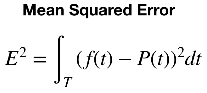
Note that the range of integral from here on is an arbitrary period of time unless specified otherwise. Here, I’m just writing it as T, but you could think of it as a full period [t, t+T].

To minimize the loss, we usually take the derivatives respect to coefficients. In this case, a’s and b’s and by setting them to zero, we can get the best coefficients that best describe the function P(t) which is the approximated version of f(t) using sines and cosines.

By solving the above derivatives, we could get coefficients a’s and b’s. So let’s start by solving a’s first.

It’s ok to use the above equation, but we could clean the equation a bit.

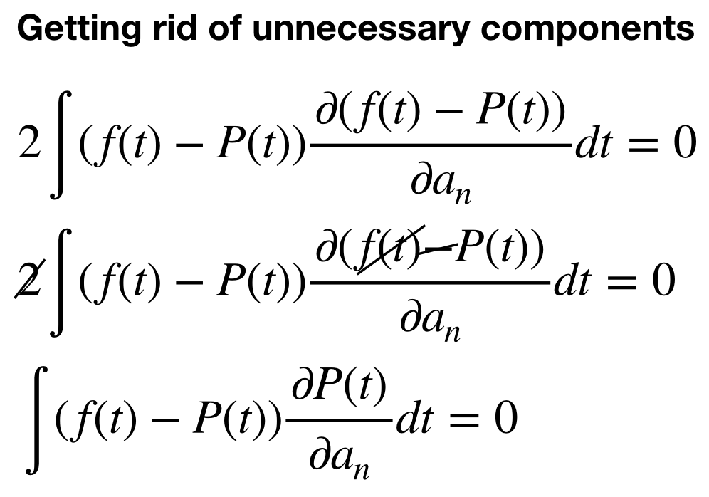
Since we don’t really need constant 2 removing it. Also, there’s no a’s in f(t) so by taking the derivative respect to a’s, we could also remove this term.

Now we are ready to move on. Let’s start from n = 0 case.

Case 1: n = 0

So now we have a simplified version of the derivative respect to a’s equals to zero:

To solve this equation, we want to know what’s the following term represent:

If you look back to check what P(t) was, we can easily calculate this derivative and get this.

Now plugging this back to the derivative = 0 equation, we get:

We could solve this left side just by simply taking the integral on each term of P(t). Note that most of the term just goes to zero if you remember what we have talked about in the orthogonal functions. (This part simply all the terms except the first one goes to zero because integration of any cosine and sine functions over a period of time is zero if you check the figure in the orthogonal function section)

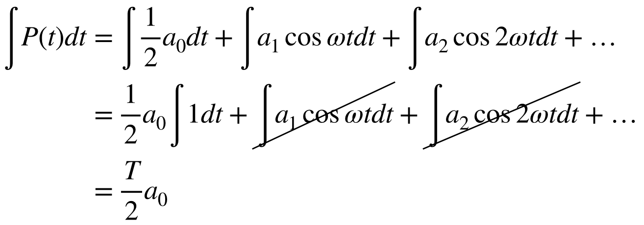
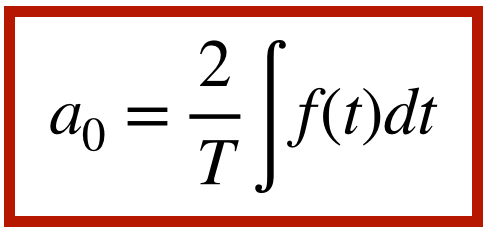
Therefore we get coefficient a_0

Case 2: n = 1

Now we do the same for n = 1. First calculate the partial derivative from P(t).

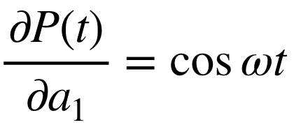
Plug it in the equation that we are trying to solve.

And by using the properties of orthogonality, we get:

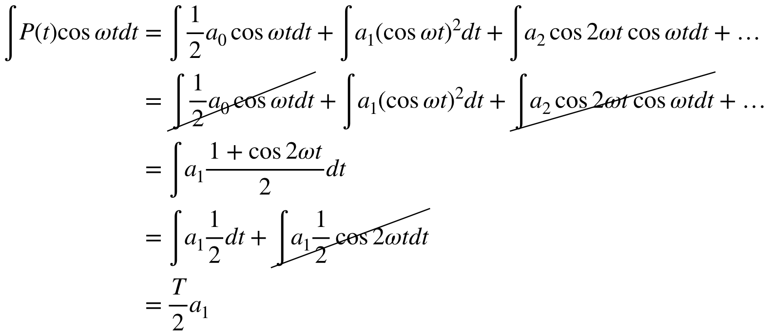
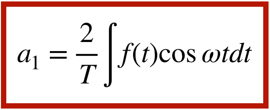
Therefore, the coefficient a_1 is

Case 3 and beyond: General a’s and b’s

So if you keep doing that for all the a’s and b’s, you will realize the general equation for a’s and b’s.

By using these equations, you can easily get coefficients that can then be plugged into the original equation of P(t).

After that, P(t) will be your approximation of f(t) as a real fourier series! Congrats!

Note that there are assumptions that the original signal f(t) has to be in the real domain and periodic function. In the next story, we are going to extend to complex fourier series where you can now even apply this to complex (imaginary) domain.

Summary

• What is Fourier Transform in general

It’s a technique to decompose signals into sine and cosine waves.

• What are the orthogonal functions

It only has a value when m = n and otherwise, it’s zero.

• Introduction to Real Fourier Series

One of the early steps before understanding the Fourier Transform. Decomposition of a periodic function using sine and cosine with coefficients applied in the real domain.