The Sheer Nonsense of the Quantity Theory of Money

It has come to my attention that many people in the crypto community use the Quantity Theory of Money’ to justify valuations of utility tokens, despite the fact that the “theory” is discredited by most professional economists as arrant nonsense.

I thought that it would be useful to provide a brief recap of the theory, and provide a crystal clear exposition of why it is completely useless as a justification for network value.

First the theory is often represented as an equation:

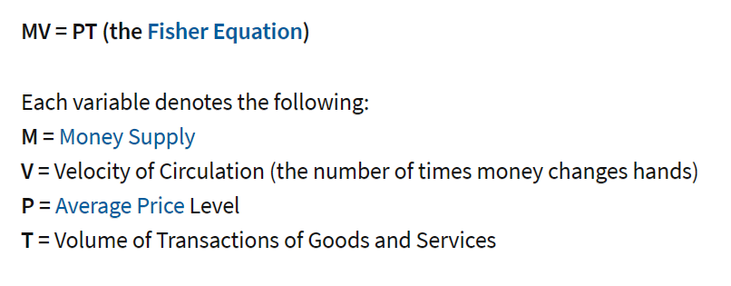
Because it is represented as an equation, many people consider that you can “solve it” for one of the variable, and therefore derive how one variable would be impacted by another (such as by increasing velocity or money supply).

However most economists would represent it as follows:

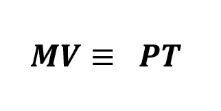
This is an entirely different representation — it states that the result is an accounting tautology and no causation can be implied (subtly because the variables are not independent but are functions of each other).

The oft used analogy is the observation of fires — we observe fires and we observe firetrucks at each fire. If we let F

And we can ‘solve’ this equation to determine the ‘cause’ of fires:

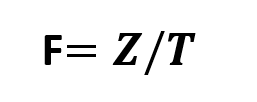
Now if we want to reduce the number of fires, it seems all we need to do is increase the number of firetrucks at each fire.

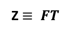
Instead the equation should have been written as an identity, and no algebra is allowed!

We can show very clearly how this works in our QTM by considering a simplified model of a network.

Assume we have a network that consists initially of five players, arranged in a circle so they can all participate with each other. Each player has a stack of marbles of different colors that they wish to trade with each other. Each exchange involves one marble being exchange for a set of coins. The price of a marble is exogenous (say because there are many tables and we are aware of the current ‘price level’. Denote the price by P. The value of coins around the table is designated by M (using the same base unit as P). If we look at our system for a unit of time (say an hour) then we can see how many transactions occur in that hour, say T (which is the ‘volume’ of transactions).

The table layout of our ‘network’ is shown below:

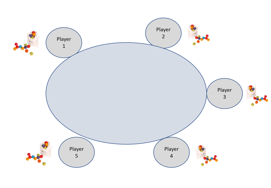
In this network we have five players who have bags of marbles that they wish to trade.

We will start the network by assuming one Player, Player 1, has the only money in the system, one coin of value P.

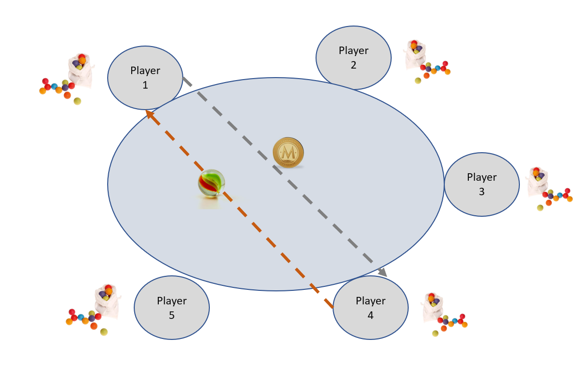
He engages in a trade with Player 4, where he exchanges one coin of value P for one marble. The transaction takes say Y minutes to complete. Because our money supply is restricted to 1 coin, M must equal P. And every transaction must be sequential — so now Player 4 can engaged with Player 3 and do an exchange, then Player 3 has the coin, so she can engage in a transaction. How many transactions can be completed in the hour? Simple — 60/Y. So we now have some simple identities in our constrained case:

M=P

T = 60/Y

V = 60/Y (with units of ‘transaction per hour’)

And MV = PT becomes:

P*60/Y = P* 60/Y

So far so good. What if we increase the number of coins (increase the money supply)? Say have every player start with one coin? But assume players can only engage in one transaction at a time. So now the maximum number of simultaneous transactions is the number of pairs. With five players we can only have two pairwise combinations at any point in time.

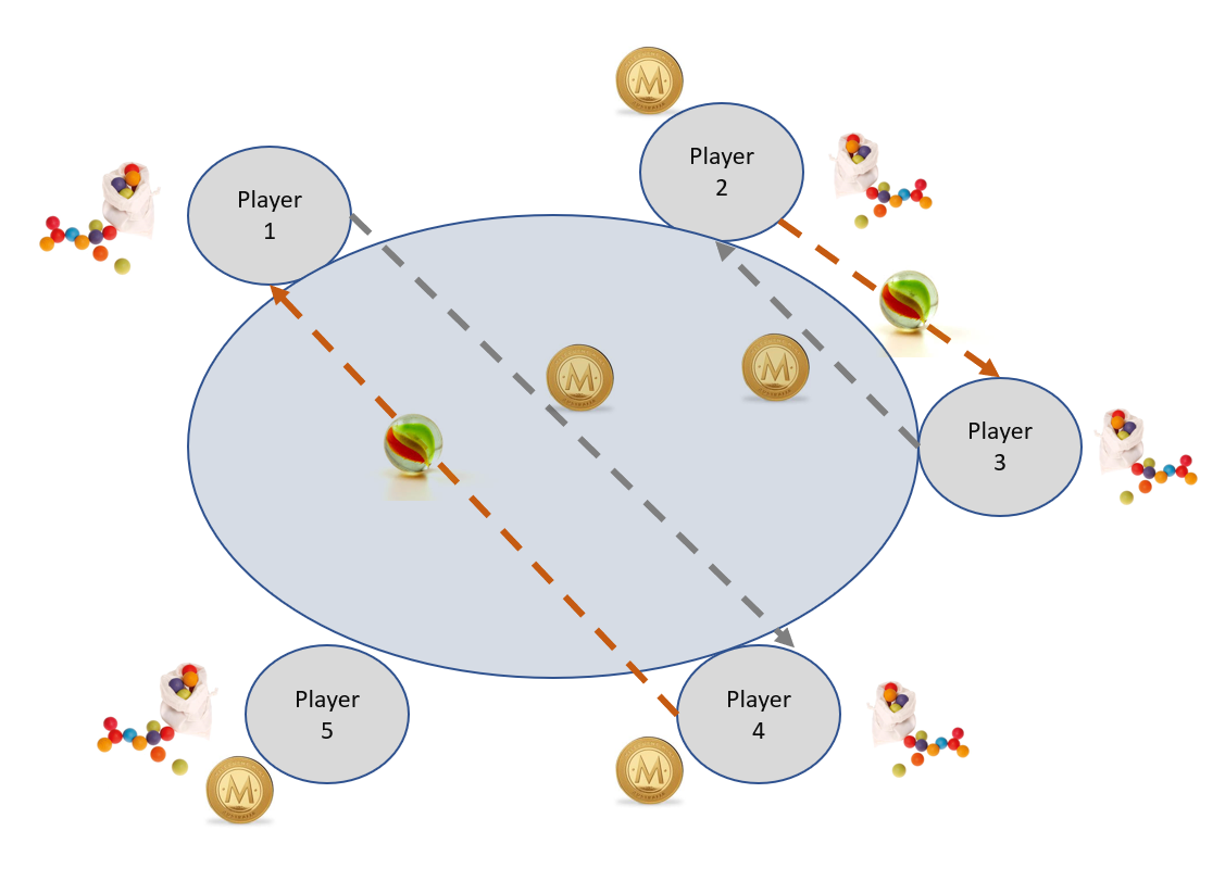
Now we have to be very careful. What is the definition of the money supply?

Is it the number of coins possessed by the players (which is five) or is it the number of coins being exchanged?

Firstly we know how many transactions can occur in the hour. It is 2*60/Y because we can double the number of transactions. So our identity for T is:

T = 2*60/Y

Our velocity is the rate at which money changes hands (which in our definition here is 60/Y:

V = 60/Y

Our ‘Money Supply’ is either 5P or 2P … depending on our definition. So if it is 5P then our equation is:

MV=PT becomes:

5*P*60/Y = P*2*60/Y which is obviously incorrect. So the real definition of ‘Money Supply’ must be the money being exchanged, not the money supplied, so now our equation is:

2*P*60/Y = P*2*60/Y

What is really going on here?

What is really happening is that each variable is not independent.

The total amount of money ‘in circulation’ is actually the number of simultaneous transactions that can occur times the amount of money involved in each transaction. So M = P*(Simultaneous Tx Rate)

Velocity is simply the rate at which transactions occur, which is 60/(Time per Tx)

The total number of transactions is simply the minutes times the Simultaneous Tx Rate divided by Time Per Transaction. Because the number of minutes in 1 hour is 60 here, T=60*(Simultaneous Tx Rate)/(Time Per Tx)

So MV=PT becomes the tautology

In other words, this is an accounting tautology where all the variables are functions of the rate and the time per transaction.

This should be bleedingly obvious but the fact that crypto specialists keep chatting about how the Quantity Theory Of Money somehow is a predictor of the price of a token is very disturbing and is indicative of a very low level of mathematical understanding.

To reiterate, using the QTM to calculate the value or the price of a token makes the fundamental mathematical mistake of treating an equivalence equation between dependent variables as the same as an algebraic equation between independent variables.

There is zero causative or descriptive power in the Quantity Theory of Money as it applies to the valuation of crypto tokens. Full stop.