A machine learning survival kit for doctors
We are ready to start with algorithms! From here things will be getting a bit more difficult, so make sure you have enough time to go through to the end :).
Defining the Problem: Predicting Y from X
A good practice in machine learning is to start with a simple baseline algorithm to get a grasp of the complexity of your problem. So, we first decided not to use the whole 3D MRIs, but a simpler reflection of their content, in the form of their histogram of voxel intensities
For a computer, an MRI is a 3D grid of values — the voxel grayscale intensity values — where low and high values are often represented as black and white, respectively. The histogram of an image is the histogram of these values. Another way to put it: it is the count of voxels that have a grayscale value within a given range. A typical histogram is shown below. On the x-axis you can see the grayscale values ranging from 0 to 1, and on the y-axis the total count of voxels for each value. Values have been grouped in small intervals, visually represented by the columns in the figure, called bins. We set the number of bins to 200, meaning the interval [0, 1] is split into 200 equally sized intervals. See our

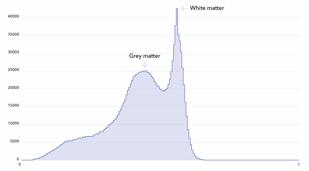
The idea is that homogeneous tissues have similar grayscale values. So to determine the quantity and proportion of grey matter and white matter, respectively, you can count the number of voxels that have similar values. Indeed, you can see on the figure that we identify 2 peaks, from left to right: grey matter (low intensity values) and white matter (high intensity values). We know that brain aging is correlated with grey matter atrophy… and grey matter quantity is related with the dimension of the first peak. Let’s explore this further!
Going back to our X and Y notations, we replaced our X with vectors (just a sequence of numbers) of length 200. In mathematical notation, for a single MRI, X= [X₁,X₂, …, X₂₀₀] where Xᵢ is the number of voxels in the i-th bin. We call this concise description of the MRI a feature vector. The main concept of machine learning algorithms is that there are not a sequence of human hand-crafted rules that indicate how to go from X to Y, but they can “learn” themselves these rules using data, i.e. a lot of examples of X and Y.This is one of the main difference between Deep Blue, the IBM chess-playing computer, and the recent AlphaGo, the first computer program able to defeat a professional Go player.
To be more precise, “training” an algorithm means searching for a function F, the algorithm, so that F(X), the prediction of the algorithm, is a close as possible to Y, the true value, for all the pairs (X, Y) of the dataset. In practice, we search F within a large family of functions (linear functions, decision trees, neural networks, etc.) and chose the one that has the minimal average error between the prediction F(X) and the true value of Y. In short, “learning” is nothing but an optimization problem: minimizing an error. In our case, we have 1597 pairs of the form (X = histogram, Y = age), and we try to minimize the absolute error |F(X) — Y|. For example, if the prediction F(X) is 23 years of age, and the true value of Y is 21 years of age, the absolute error is 2 years. If you understand this paragraph, you understand supervised machine learning.
Cross-validation: splitting training and test sets
We now arrive at one of the most crucial steps of the machine learning workflow : how can we evaluate the efficiency of an algorithm ? The fundamental machine-learning technique addressing this question is called cross-validation. We randomly split our dataset in two parts: a training set and a test set (also called validation set). The training set is used to train the algorithm, and the test set is only used to compute its performance. The idea is to evaluate how well the algorithm generalizes on new data it never saw during training, making the test set a proxy to evaluate the performance on new real world data. Each time we report an absolute error in this article, it is the error on the test set, and never on the training set.
A difficult question we have to ask ourselves is how to determine the relative proportions of the training set and the test set. 50/50? 75/25? 90/10? The larger the training set, the better the algorithm because it is trained on more data. However, a larger test set implies more reliable performance, as the data becomes more representative of the real world.
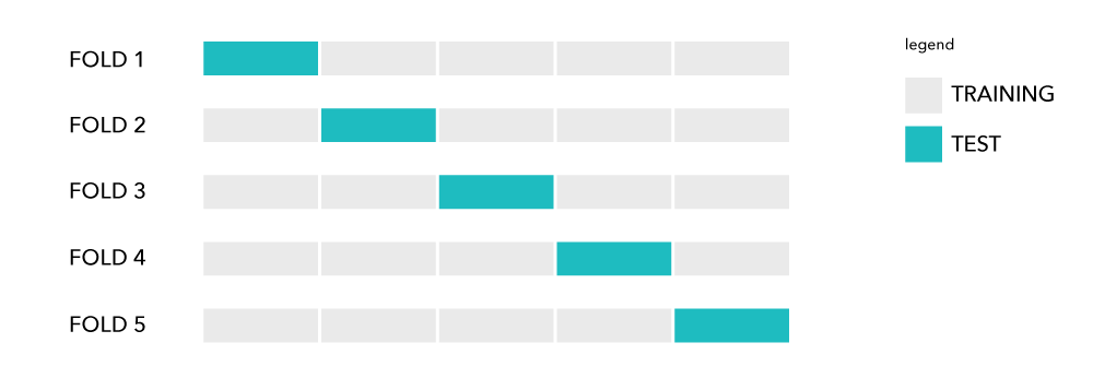
We used a procedure called k-fold cross-validation: we randomly split the dataset in 5 chunks, or folds, of equal size, and repeat the training 5 times, each time taking a different fold as the test set and the four others as train set (equivalent to a 80/20 split). This forces us to train and test the algorithm 5 times, which can take hours, but it makes the results much more reliable. However, since these fold evaluations are independent, evaluating the cross-validation performance parallelizes easily (if you have the computational resources available).

In medical studies cross-validation is often not enough. Commonly, results reported in papers are over-estimated, as one may iterate many times over the same dataset to obtain the best cross-validated performance. Therefore, it is best practice to validate an algorithm on an external independent dataset, provided by another institution or hospital. Lack of transferability from an hospital to another, or from a population to another, may be a major flaw of machine learning algorithms, but so far there is no equivalent of clinical trials for AI algorithms imposed by the FDA or equivalents.
Finding the right model
Linear models
There exist a large variety models, i.e. families of functions F, and choosing the right one for your problem of interest requires some experience. Again, a good practice is to begin with the simplest effective method, and for this, linear models are always a good baseline.
In a linear model, the prediction F(X) is a weighted sum of the values of X: F(X) = (W₁ * X₁) + (W₂ * X₂) + … + (W₂₀₀ * X₂₀₀) + β, where Wᵢ is a “weight” associated to the value of feature Xᵢ, and β is some constant additive term often called the bias. For instance, if X₁₂₀ corresponds to the bin of the grey matter peak, one possible (very) simple linear model that correlates the predicted age with the amount of grey matter in the MRI might be F(X) = 100+(-10 * X₁₂₀) , where β = 100, W₁₂₀ = -10, and all other Wᵢ = 0. This function seems to make sense: the more grey matter (large X₁₂₀), the lower the age.
In the case of linear regression, simple algebra performed on the training data will help us find the best possible weights Wᵢ. We used the Scikit Learn Python package to train our linear models over our 5 cross-validation subset folds. Try it yourself in our Colab notebook!
Training a linear model on the MRI intensity histogram feature vectors gives us mean absolute errors (in years) of 8.49, 9.53, 9.29, 8.89, and 9.22 on each of the 5 folds, so an average error of 9.08 years. It is not great…but not that bad either! With this extremely simple algorithm, we can predict from brain scans whether a patient is younger or older than 50 years of age with an accuracy of 84%.
Non-linear models
The hypothesis of a linear relation between an MRI histogram and the age is, of course, simplistic. An algorithm taking into account a non-linear relationship may be able to provide more accurate predictions. Gradient tree boosting is one of the most popular and efficient non-linear choices for F(X). Gradient boosted trees are a sequence of decision trees iteratively built to minimize the error. You can find a more complete introduction here.
While deep neural networks, and their ability to tackle complex tasks, are nowadays oft-publicized in popular science articles and well-known even outside the machine learning community, gradient tree boosting remains less well-known outside of the data science community. Gradient boosting trees are often a key part of the winning solutions in international data science competitions organized on platforms such as Kaggle or Dream, and often are extremely hard to beat.
Using the CatBoost Python library, we get a much better result: our mean absolute error can be reduced to just 5.71 years, which is already closer to state-of-the art performance (4.16 years as reported in Cole et al. 2017). We may be tempted to stop here, publish our algorithm and validate it in clinics. But wait! We are making a large mistake which is, unfortunately, quite common… even in peer-reviewed litterature.
Avoiding a common pitfall
As mentioned earlier, the range of intensities of the voxels in MRIs has no biological meaning and varies greatly from one MRI scanner to another. In the cross-validation procedure, we randomly split subjects between the training and the test set. So, for each hospital, there will be on average 80% of images from this hospital in the training set and 20% in the test set. But what would be the consequence of focusing on randomizing not the subjects but the hospitals, and consequently the MRI scanner? In this hospital split setting, the test set would contain not just new patients, but data from scanners never seen during training.
Once we split by hospital, the mean absolute error of our linear regression and gradient tree boosting models increase by around 5 and 6 years, up to 14.22 and 11.52 years error. Even a naive algorithm, F(X)=27, that predicts all MRIs to be from subjects of 27 years of age (the median age of the dataset) would get an average error of around 14 years. Our trained algorithms do not seem to perform much better than reporting the median of the dataset in the case of the hospital split. Somehow, in the random split setting, our algorithms must have been able to use the fact that a subject came from a given hospital to accurately predict its age.
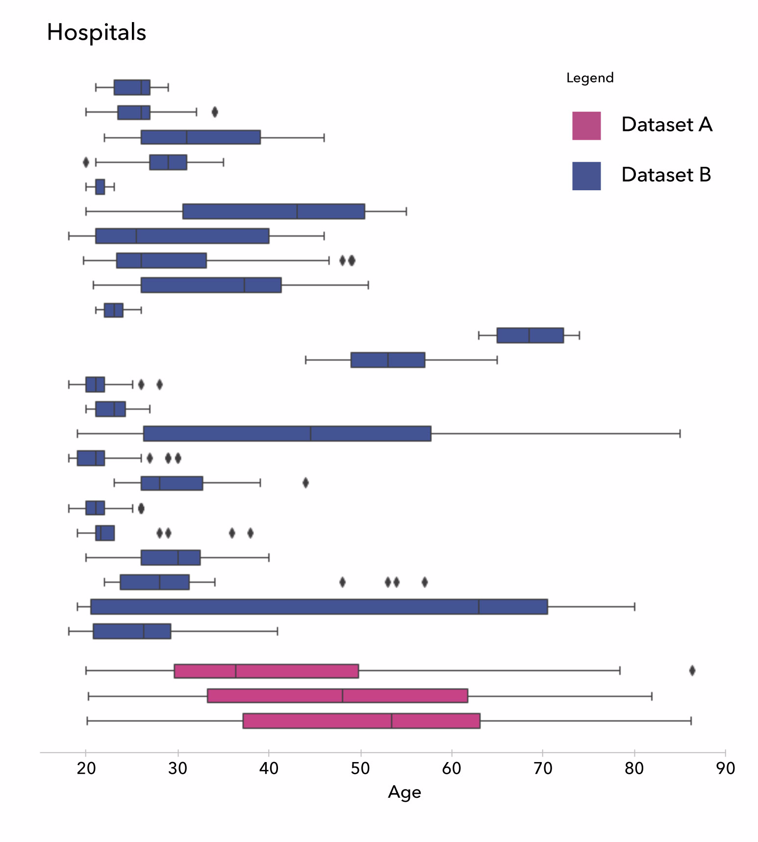
The following figures show that a more careful data analysis would have prevented us from making such a mistake. You can see on this first figure that the distribution of the ages per hospital: most hospitals have a bias in their recruitment. Some have only young subjects in their datasets, some others only old ones.

In the next figure, we show the averaged the histograms of the subjects in each hospital, with each curve representing a different hospital.

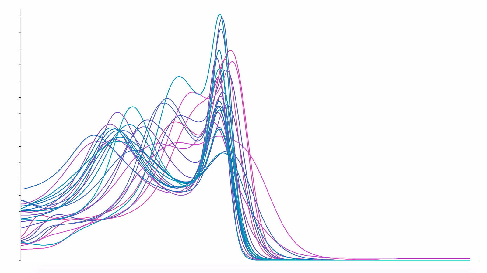
And here we get our answer: while the white matter peaks are quite aligned across MRIs sourced from different hospitals, the grey matter peaks are spread wide from hospital to hospital due to the use of different scanners. Because of this feature, it is was quite easy for the algorithms to 1) detect the source hospital using the histogram and 2) use this information to constrain the age prediction to the range of ages recorded in the dataset provided by this hospital.
To remove this effect, we decided to go back on the last step of our preprocessing pipeline: the intensity normalization procedure. We moved from the white stripe normalization (method v1), which only fixes the white matter peak, to a new home-made method (method v2) that additionally fixes the grey matter peak. So now, the white matter and grey matter signals are centered on fixed values, and indeed the per-hospital average histograms now look much better, as shown in the next figure.

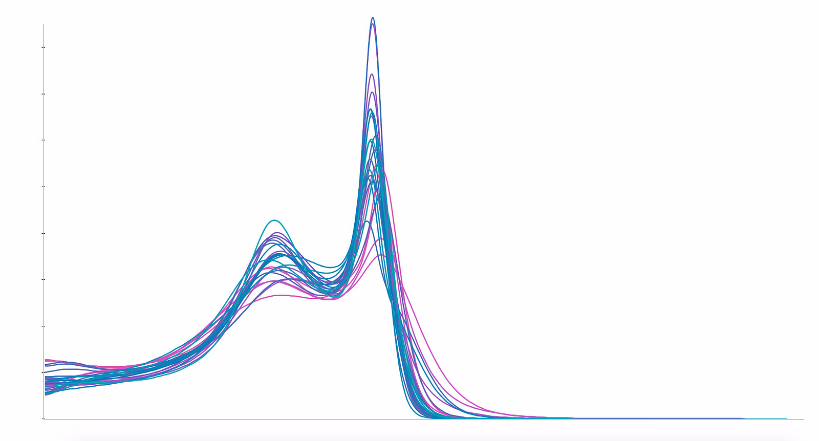
As expected, when we re-run the linear and non-linear models, we get much better results when using cross-validation over hospital splits. We still observe that the non-linear gradient boosting models are more powerful than the baseline linear regression.

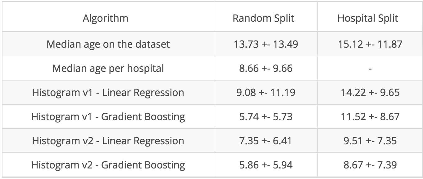
Note that looking at a random split is not necessarily irrelevant. After all, you may be happy to have an algorithm which is able to take into account the specificities of the scanner the image comes from, as long as it does not integrate selection bias from the hospital.
Main Takeaways
- Spend time to analyze your data.
- Begin with simple approaches as baselines.
- Non-linear models can be a powerful tool if used properly.
- Be very careful with cross-validation in multi-centric studies, when you have several samples per patient, or when you have a small sample size. Best practice is to have an external and independent validation set. Splitting data is not always as easy as it sounds…
