In this tutorial we will discuss about Maximum Entropy text classifier, also known as MaxEnt classifier. The Max Entropy classifier is a discriminative classifier commonly used in Natural Language Processing, Speech and Information Retrieval problems. Implementing Max Entropy in a standard programming language such as JAVA, C++ or PHP is non-trivial primarily due to the numerical optimization problem that one should solve in order to estimate the weights of the model.

Update: The Datumbox Machine Learning Framework is now open-source and free to download. Check out the package com.datumbox.framework.machinelearning.classification to see the implementation of Max Entropy Classifier in Java.

Note that Max Entropy classifier performs very well for several Text Classification problems such as

Sentiment Analysis and it is one of the classifiers that is commonly used to power up our Machine Learning API.

What is the Max Entropy Classifier?

The Max Entropy classifier is a probabilistic classifier which belongs to the class of exponential models. Unlike the Naive Bayes classifier that we discussed in the previous article, the Max Entropy does not assume that the features are conditionally independent of each other. The MaxEnt is based on the

Principle of Maximum Entropy and from all the models that fit our training data, selects the one which has the largest entropy. The Max Entropy classifier can be used to solve a large variety of text classification problems such as language detection, topic classification, sentiment analysis and more.

When to use the MaxEnt Text Classifier?

Due to the minimum assumptions that the Maximum Entropy classifier makes, we regularly use it when we don’t know anything about the prior distributions and when it is unsafe to make any such assumptions. Moreover Maximum Entropy classifier is used when we can’t assume the conditional independence of the features. This is particularly true in Text Classification problems where our features are usually words which obviously are not independent. The Max Entropy requires more time to train comparing to Naive Bayes, primarily due to the optimization problem that needs to be solved in order to estimate the parameters of the model. Nevertheless, after computing these parameters, the method provides robust results and it is competitive in terms of CPU and memory consumption.

Theoretical Background of Maximum Entropy

Our target is to use the contextual information of the document (unigrams, bigrams, other characteristics within the text) in order to categorize it to a given class (positive/neutral/negative, objective/subjective etc). Following the standard bag-of-words framework that is commonly used in natural language processing and information retrieval, let {w₁,…,w_m} be the m words that can appear in a document. Then each document is represented by a sparse array with 1s and 0s that indicate whether a particular word w_i exists or not in the context of the document. This approach was proposed by Bo Pang and Lillian Lee (2002).

Our target is to construct a stochastic model, as described by Adam Berger (1996), which accurately represents the behavior of the random process: take as input the contextual information x of a document and produce the output value y. As in the case of Naive Bayes, the first step of constructing this model is to collect a large number of training data which consists of samples represented on the following format: (x_i,y_i) where the x_i includes the contextual information of the document (the sparse array) and y_i its class. The second step is to summarize the training sample in terms of its empirical probability distribution:

[1]

Where N is the size of the training dataset.

We will use the above empirical probability distribution in order to construct the statistical model of the random process which assigns texts to a particular class by taking into account their contextual information. The building blocks of our model will be the set of statistics that come from our training dataset i.e. the empirical probability distribution.

We introduce the following indicator function:

[2]

We call the above indicator function as “feature”. This binary valued indicator function returns 1 only when the class of a particular document is c_i and the document contains the word w_k.

We express any statistic of the training dataset as the expected value of the appropriate binary-valued indicator function f_j. Thus the expected value of feature f_j with respect to the empirical distribution  is equal to:

[3]

If each training sample (x,y) occurs once in training dataset then  is equal to 1/N.

When a particular statistic is useful to our classification, we require our model to accord with it. To do so, we constrain the expected value that the model assigns to the expected value of the feature function f_j. The expected value of feature f_j with respect to the model  is equal to:

[4]

Where  is the empirical distribution of x in the training dataset and it is usually set equal to 1/N.

By constraining the expected value to be the equal to the empirical value and from equations [3],[4] we have that:

[5]

Equation [5] is called constrain and we have as many constrains as the number of j feature functions.

The above constrains can be satisfied by an infinite number of models. So in order to build our model, we need to select the best candidate based on a specific criterion. According to the principle of Maximum Entropy, we should select the model that is as close as possible to uniform. In order words, we should select the model p* with Maximum Entropy:

[6]

Given that:

1. [7]
2. [8]
3. [9]

To solve the above optimization problem we introduce the Lagrangian multipliers, we focus on the unconstrained dual problem and we estimate the lamda free variables {λ₁,…,λ_n} with the Maximum Likelihood Estimation method.

It can be proven that if we find the {λ₁,…,λ_n} parameters which maximize the dual problem, the probability given a document x to be classified as y is equal to:

[10]

Thus given that we have found the lamda parameters of our model, all we need to do in order to classify a new document is use the “maximum a posteriori” decision rule and select the category with the highest probability.

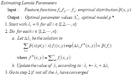
Estimating the lamda parameters requires using an iterative scaling algorithm such as the GIS (Generalized Iterative Scaling) or the IIS (Improved Iterative Scaling).

The  is the total number of features which are active for a particular (x,y) pair. If this number is constant for all documents then the  can be calculated in closed-form:

[11]

The assumption that  is constant is rarely realistic in practice. To resolve this, some versions of IIS propose the inclusion of a “slack” indicator function that helps maintaining the number of active features constant. Unfortunately, introducing such a feature heavily increases the training time. Fortunately, as Goodman (2002) and Ratnaparkhi (1997)prove, it is only necessary that the sum of indicator functions to be bounded by and not necessarily equal to it. Thus we can select as C the maximum number of active features for all (x,y) pairs within our training dataset:

 [16]

Making the above adaptations on the standard versions of IIS can help us find the {λ₁,…,λ_n} parameters and build our model relatively quickly.

As we discussed in the previous article “The importance of Neutral Class in Sentiment Analysis”, Max Entropy classifier has few very nice properties when we use it on Sentiment Analysis and when we include the Neutral Class. If you want to check out some applications of Max Entropy in action, check out our Sentiment Analysis or Subjectivity Analysis API. To use our API just sign-up for a free account and get your API Key from your profile area.

Did you like the article? Please take a minute to share it on Twitter.