Binary Search Tree: Coding Mode On

Now it’s coding time! What will we see here? Insertion, search for a value, deletion, and balance the tree. Let’s the game begin

Insertion: adding new nodes to our tree

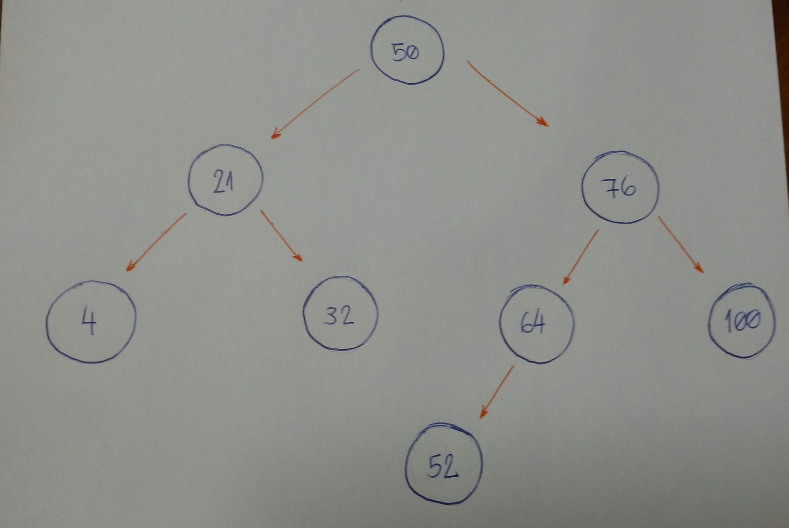
Imagine we have an empty tree and we want to start adding new nodes with these values: 50, 76, 21, 4, 32, 100, 64, 52. In that order.

The first thing we need to know is 50 is the root of our tree.

So now we can start inserting node by node.

• 76: greater than 50, insert on the right side.
• 21: smaller than 50, insert on the left side.
• 4: smaller than 50. Node with value 50 has a left child (21). 4 is smaller than 21, insert it on the left side of this node
  .
• 32: smaller than 50. Node with value 50 has a left child (21). 32 is greater than 21, insert it on the right side of this node.
• 100: greater than 50. Node with value 50 has a right child (76). 100 is greater than 76, insert it on the right side of this node.
• 64: greater than 50. Node with value 50 has a right child
  (76). 64 is smaller than 76, insert it on the left side of this node.
• 52: greater than 50. Node with value 50 has a right child (76). 52 is smaller than 76. Node with value 76 has a left child (64). 52 is smaller than 64, insert it on the left side of this node.

Did you notice a pattern here? Let’s break it down.

1. Ask “Is the new node value greater or smaller than the current node?”
2. Is the new node value greater than the current node? Go to the right subtree. If the current node doesn’t have a right child, insert it there. Else backtrack to rule number 1.
3. Is the new node value smaller than the current node? Go to the left subtree. If the current node doesn’t have a left child, insert it there. Else backtrack to rule number 1.
4. Special case we didn’t handle: when new node value is equal to the current node‘s value. Just use the rule number 3. Consider equal values to insert in the left subtree part.

Now the code! yey!

It seems very simple. The powerful part of this algorithm is the recursion part: line 9 and line 13. Both lines of code call the insert_node method, for its left and right children, respectively. Lines 11 and 15 are the ones that we do the insertion for each child.

Searching: let’s find the node value. Or not

The algorithm that we will build now is all about searching. For a given value (integer number), we will say if our Binary Search Tree has or hasn’t that value.

One important part is how we defined the tree insertion algorithm. First we have our root node. All the left subtree nodes will have smaller values than the root node. And all the right subtree nodes will have greater values than the root node.

Example time! Imagine we have this tree.

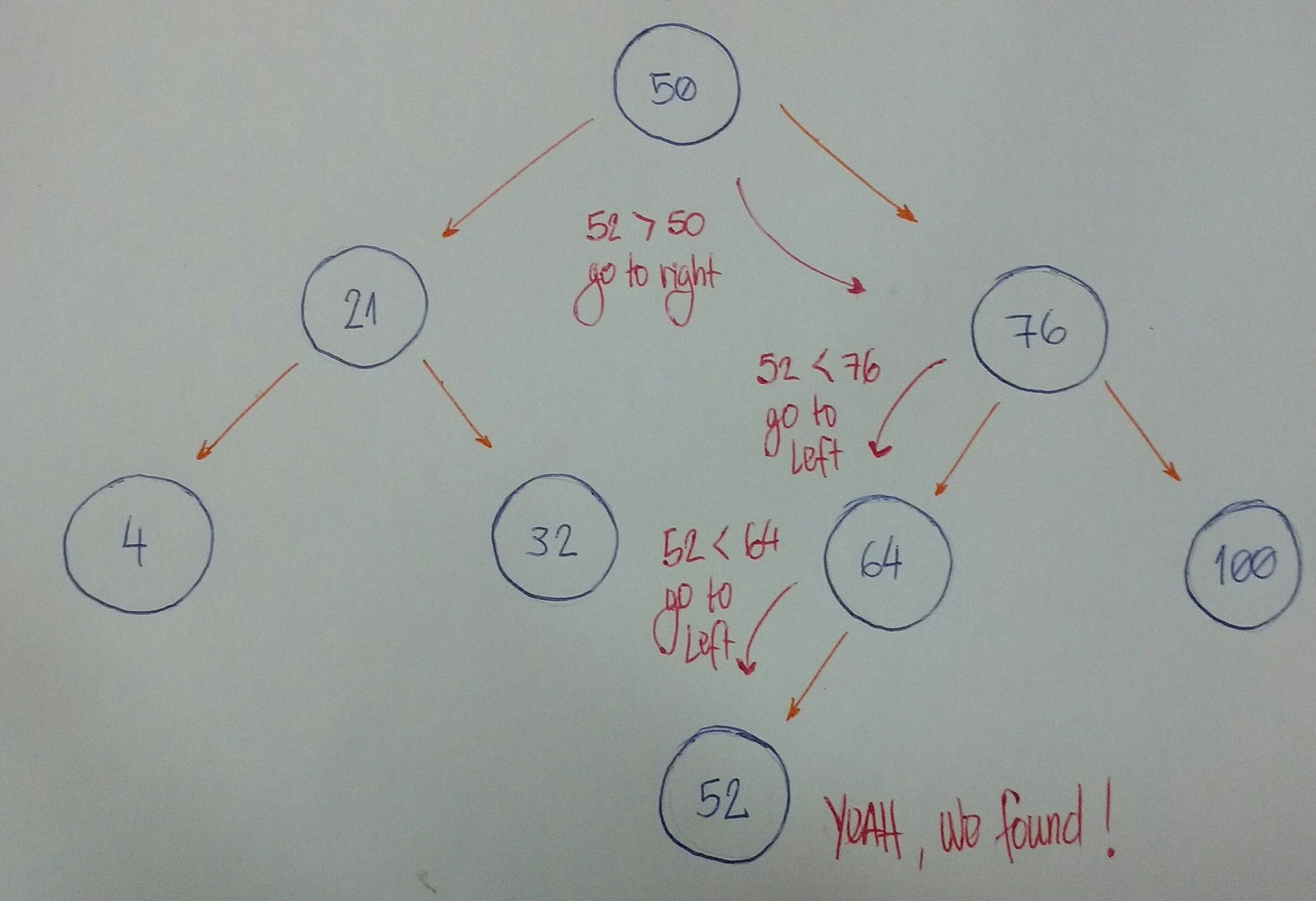
Now we want to know if we find a node based on a given value 52.

Let’s break it down.

1. We start with the root node as our current node. Is the given value smaller than the current node value? If yes, then we will search it on the left subtree.
2. Is the given value greater than the current node value? If yes, then we will search it on the right subtree.
3. If rules number 1 and number 2 are both false, we can compare the current node value and the given value if they are equal. If the return of the comparison is true then “Yeah! Our tree has the given value”. Else “Nooo. It hasn’t”.

Coding time!

• Lines 8 and 9 are the rule number 1.
• Lines 10 and 11 are the rule number 2.
• Line 13 is the rule number 3.

How do we test it?

Let’s create our Binary Search Tree initializing the root node with the value 15.

And now we will insert a lot of new nodes there.

For each inserted node we will test if our find_node method really works.

Yeah, it works for these given values! Let’s test for a value that doesn’t exist in our Binary Search Tree.

Oh yeah! Searching… done!

Deletion: removing and organizing

Deletion is a more complex algorithm, because we need to handle different cases. For a given value, we need to remove the node with this value. Imagine that this node has not children, or a single child, or two children.

• Case 1: A node with no children (leaf node).

If the node we want to delete has no children, we simply delete it. The algorithm doesn’t need to reorganize the tree.

• Case 2: A node with just one child (left or right child).

To cover the second case, our algorithm needs to make the node’s parent points to the node‘s child. If the node is the left child of its parent, we make the node’s parent left child points to the node‘s child. If the node is the right child of its parent, we make the node’s parent right child points to the node‘s child.

• Case 3: A node with two children.

When the node has 2 children, we need to find the node with the minimum value starting from the node‘s right child. We will put this node with minimum value in the place of the node we want to remove.

Coding time!

1. First thing: the parameters. value and parent. We want to find the node that has this value and the node’s parent is a important part to remove the node.
2. Second thing: the returning value. Our algorithm will return a boolean value. True if it found the node and removed it. Otherwise False.
3. From line 2 to line 9: we start searching for the node that has the value we are looking for. If the value is smaller than the current node value we go to the left subtree, recursively (if and only if the current node has a left child). If the value is greater, go to the right subtree, recursively.
4. Line 10: we start to think about the remove algorithm.
5. From line 11 to line 13: we cover the node with no children and it is the left child from its parent. We remove the node by setting the parent’s left child to None.
6. Lines 14 and 15: we cover the node with just no children and it is the right child from its parent. We remove the node by setting the parent’s right child to None.
7. Clear node method: I will show the clear_node code below. But basically it set the node left child, right child, and its value to None.
8. From line 16 to line 18: we cover the node with just one child (left child) and it is the left child from its parent. We set the parent's left child to the node’s left child (the only child it has).
9. From line 19 to line 21: we cover the node with just one child (left child) and it is the right child from its parent. We set the parent's right child to the node’s left child (the only child it has).
10. From line 22 to line 24: we cover the node with just one child (right child) and it is the left child from its parent. We set the parent's left child to the node’s right child (the only child it has).
11. From line 25 to line 27: we cover the node with just one child (right child) and it is the right child from its parent. We set the parent's right child to the node’s right child (the only child it has).
12. From line 28 to line 30: we cover the node with both left and right children. We get the node with the smallest value (code below!) and set it to the current node‘s value. Finish it by removing the smallest node.
13. Line 32: if we found the node we are looking for, we need to return True. From line 11 to line 31 we handle this case. So just return True and that’s it!