第3章 特徵選擇與特徵工程
阿新 • • 發佈:2019-01-05
標籤編碼,字典向量化,特徵雜湊
LabelEncoder和OneHotEncoder 在特徵工程中的應用
對於性別,sex,一般的屬性值是male和female。兩個值。那麼不靠譜的方法直接用0表示male,用1表示female 了。所以要用one-hot編碼。
array([[0., 1.],
       [1., 0.],
       [0., 1.],
       [0., 1.],
       [1., 0.],
       [1., 0.]])
classes_:
Holds the label for each class
>>> from from Label encoding
[0 0 0 1 0 1 1 0 0 1]
Label decoding
['Male', 'Female', 'Male', 'Male', 'Female', 'Female']
Label binarization
[[0]
[0]
[0]
[1]
[0]
[1]
[1]
[0]
[0]
[1]]
Label decoding
Dictionary data vectorization
[[10. 15. 0. 0.]
[-5. 0. 22. 0.]
[ 0. 0. -2. 10.]]
Vocabulary:
{'feature_1': 0, 'feature_2': 1, 'feature_3': 2, 'feature_4': 3}
Feature hashing
Feature decoding
[[0. 0. 0. ... 0. 0. 0.]
[0. 0. 0. ... 0. 0. 0.]
[0. 0. 0. ... 0. 0. 0.]]
[[1., 0., 0., 1., 0., 0., 0., 1., 0.]
[0., 1., 0., 0., 1., 0., 0., 0., 1.]
[0., 1., 1., 0., 0., 0., 0., 1., 0.]
[1., 0., 0., 0., 0., 1., 0., 1., 0.]
[1., 0., 0., 0., 0., 0., 1., 0., 1.]]
處理缺失資料
from __future__ import print_function

import numpy as np

from sklearn.preprocessing import Imputer

# For reproducibility
np.random.seed(1000)


if __name__ == '__main__':
    data = np.array([[1, np.nan, 2], [2, 3, np.nan], [-1, 4, 2]])
    print(data)

    # Imputer with mean-strategy
    print('Mean strategy')
    imp = Imputer(strategy='mean')
    print(imp.fit_transform(data))

    # Imputer with median-strategy
    print('Median strategy')
    imp = Imputer(strategy='median')
    print(imp.fit_transform(data))

    # Imputer with most-frequent-strategy
    print('Most-frequent strategy')
    imp = Imputer(strategy='most_frequent')
    print(imp.fit_transform(data))
[[ 1. nan  2.]
 [ 2.  3. nan]
 [-1.  4.  2.]]
Mean strategy
[[ 1.   3.5  2. ]
 [ 2.   3.   2. ]
 [-1.   4.   2. ]]
Median strategy
[[ 1.   3.5  2. ]
 [ 2.   3.   2. ]
 [-1.   4.   2. ]]
Most-frequent strategy
[[ 1.  3.  2.]
 [ 2.  3.  2.]
 [-1.  4.  2.]]
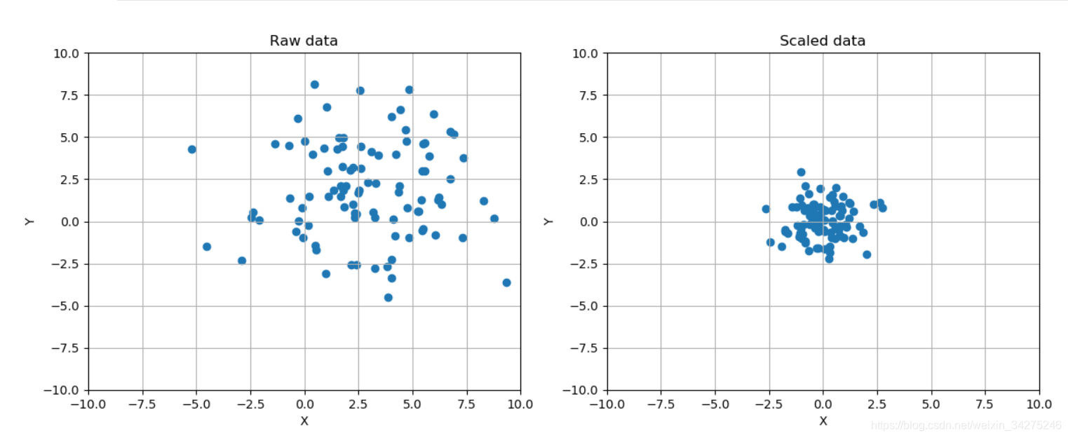
資料標準化
標準化(Standardization):對資料的分佈的進行轉換,使其符合某種分佈(比如正態分佈)的一種非線性特徵變換。
method
2.1 Rescaling (min-max normalization)
2.2 Mean normalization
2.3 Standardization
2.4 Scaling to unit length
from __future__ import print_function

import numpy as np
import matplotlib.pyplot as plt

from sklearn.preprocessing import StandardScaler, RobustScaler

# For reproducibility
np.random.seed(1000)

if __name__ == '__main__':
    # Create a dummy dataset
    data = np.ndarray(shape=(100, 2))

    for i in range(100):
        data[i, 0] = 2.0 + np.random.normal(1.5, 3.0)
        data[i, 1] = 0.5 + np.random.normal(1.5, 3.0)

    # Show the original and the scaled dataset
    fig, ax = plt.subplots(1, 2, figsize=(14, 5))

    ax[0].scatter(data[:, 0], data[:, 1])
    ax[0].set_xlim([-10, 10])
    ax[0].set_ylim([-10, 10])
    ax[0].grid()
    ax[0].set_xlabel('X')
    ax[0].set_ylabel('Y')
    ax[0].set_title('Raw data')

    # Scale data
    ss = StandardScaler()
    scaled_data = ss.fit_transform(data)

    ax[1].scatter(scaled_data[:, 0], scaled_data[:, 1])
    ax[1].set_xlim([-10, 10])
    ax[1].set_ylim([-10, 10])
    ax[1].grid()
    ax[1].set_xlabel('X')
    ax[1].set_ylabel('Y')
    ax[1].set_title('Scaled data')

    plt.show()

    # Scale data using a Robust Scaler
    fig, ax = plt.subplots(2, 2, figsize=(8, 8))

    ax[0, 0].scatter(data[:, 0], data[:, 1])
    ax[0, 0].set_xlim([-10, 10])
    ax[0, 0].set_ylim([-10, 10])
    ax[0, 0].grid()
    ax[0, 0].set_xlabel('X')
    ax[0, 0].set_ylabel('Y')
    ax[0, 0].set_title('Raw data')

    rs = RobustScaler(quantile_range=(15, 85))
    scaled_data = rs.fit_transform(data)

    ax[0, 1].scatter(scaled_data[:, 0], scaled_data[:, 1])
    ax[0, 1].set_xlim([-10, 10])
    ax[0, 1].set_ylim([-10, 10])
    ax[0, 1].grid()
    ax[0, 1].set_xlabel('X')
    ax[0, 1].set_ylabel('Y')
    ax[0, 1].set_title('Scaled data (15% - 85%)')

    rs1 = RobustScaler(quantile_range=(25, 75))
    scaled_data1 = rs1.fit_transform(data)

    ax[1, 0].scatter(scaled_data1[:, 0], scaled_data1[:, 1])
    ax[1, 0].set_xlim([-10, 10])
    ax[1, 0].set_ylim([-10, 10])
    ax[1, 0].grid()
    ax[1, 0].set_xlabel('X')
    ax[1, 0].set_ylabel('Y')
    ax[1, 0].set_title('Scaled data (25% - 75%)')

    rs2 = RobustScaler(quantile_range=(30, 65))
    scaled_data2 = rs2.fit_transform(data)

    ax[1, 1].scatter(scaled_data2[:, 0], scaled_data2[:, 1])
    ax[1, 1].set_xlim([-10, 10])
    ax[1, 1].set_ylim([-10, 10])
    ax[1, 1].grid()
    ax[1, 1].set_xlabel('X')
    ax[1, 1].set_ylabel('Y')
    ax[1, 1].set_title('Scaled data (30% - 60%)')

    plt.show()
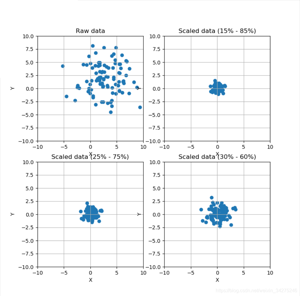
Compare the effect of different scalers on data with outliers
資料歸一化
歸一化:對資料的數值範圍進行特定縮放,但不改變其資料分佈的一種線性特徵變換。
1.min-max 歸一化:將數值範圍縮放到(0,1),但沒有改變資料分佈;
2.z-score 歸一化:將數值範圍縮放到0附近, 但沒有改變資料分佈;
from __future__ import print_function

import numpy as np

from sklearn.preprocessing import Normalizer

# For reproducibility
np.random.seed(1000)

if __name__ == '__main__':
    # Create a dummy dataset
    data = np.array([1.0, 2.0, 8])
    print(data)

    # Max normalization
    n_max = Normalizer(norm='max')
    nm = n_max.fit_transform(data.reshape(1, -1))
    print(nm)

    # L1 normalization
    n_l1 = Normalizer(norm='l1')
    nl1 = n_l1.fit_transform(data.reshape(1, -1))
    print(nl1)

    # L2 normalization
    n_l2 = Normalizer(norm='l2')
    nl2 = n_l2.fit_transform(data.reshape(1, -1))
    print(nl2)
[1. 2. 8.]
[[0.125 0.25  1.   ]]
[[0.09090909 0.18181818 0.72727273]]
[[0.12038585 0.24077171 0.96308682]]
特徵篩選
from __future__ import print_function

import numpy as np

from sklearn.datasets import load_boston, load_iris
from sklearn.feature_selection import SelectKBest, SelectPercentile, chi2, f_regression

# For reproducibility
np.random.seed(1000)

if __name__ == '__main__':
    # Load Boston data
    regr_data = load_boston()
    print('Boston data shape')
    print(regr_data.data.shape)

    # Select the best k features with regression test
    kb_regr = SelectKBest(f_regression)
    X_b = kb_regr.fit_transform(regr_data.data, regr_data.target)
    print('K-Best-filtered Boston dataset shape')
    print(X_b.shape)
    print('K-Best scores')
    print(kb_regr.scores_)

    # Load iris data
    class_data = load_iris()
    print('Iris dataset shape')
    print(class_data.data.shape)

    # Select the best k features using Chi^2 classification test
    perc_class = SelectPercentile(chi2, percentile=15)
    X_p = perc_class.fit_transform(class_data.data, class_data.target)
    print('Chi2-filtered Iris dataset shape')
    print(X_p.shape)
    print('Chi2 scores')
    print(perc_class.scores_)
Boston data shape
(506, 13)
K-Best-filtered Boston dataset shape
(506, 10)
K-Best scores
[ 88.15124178  75.2576423  153.95488314  15.97151242 112.59148028
 471.84673988  83.47745922  33.57957033  85.91427767 141.76135658
 175.10554288  63.05422911 601.61787111]
Iris dataset shape
(150, 4)
Chi2-filtered Iris dataset shape
(150, 1)
Chi2 scores
[ 10.81782088   3.59449902 116.16984746  67.24482759]
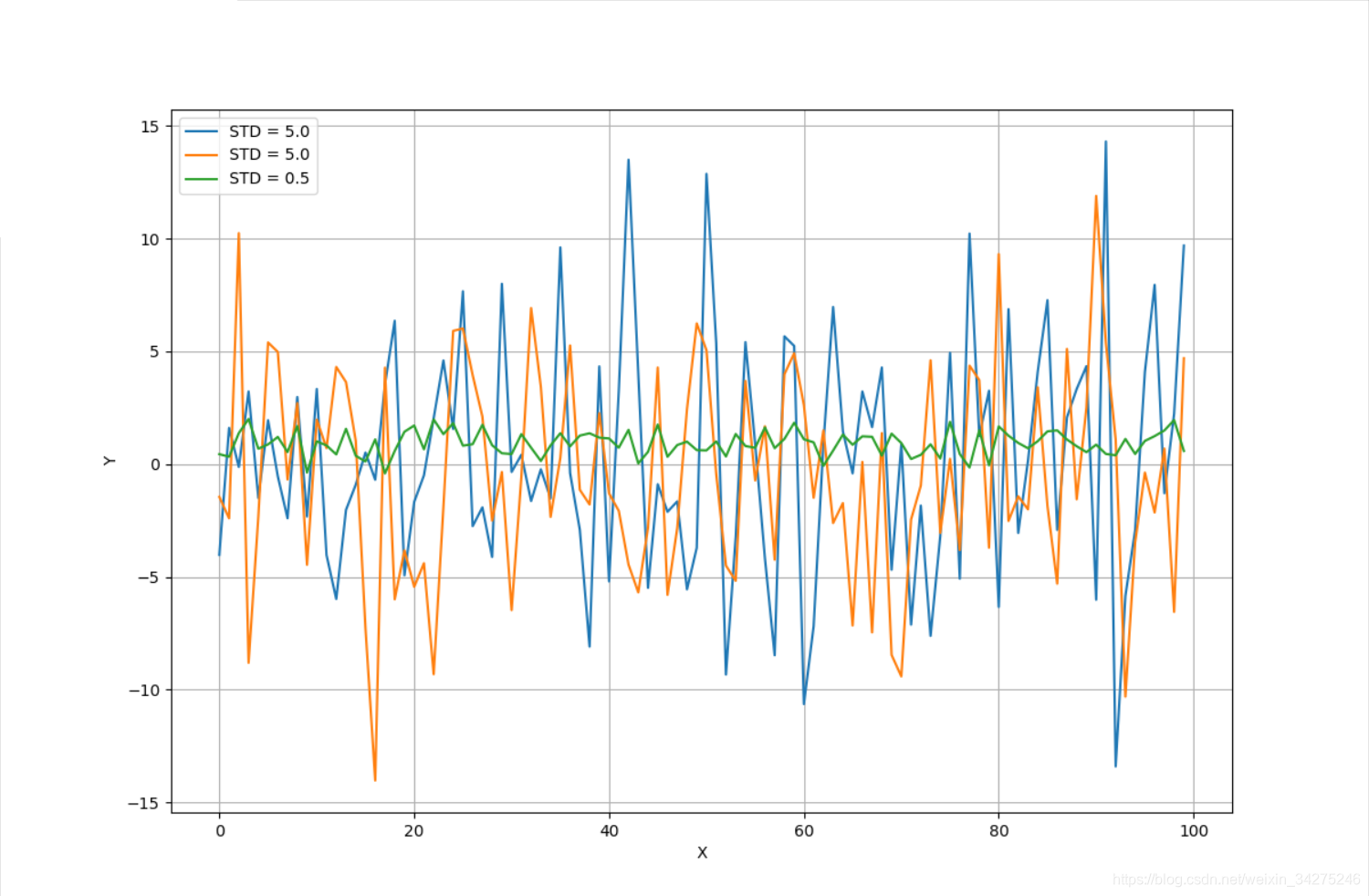
特徵選擇
from __future__ import print_function

import numpy as np
import matplotlib.pyplot as plt

from sklearn.feature_selection import VarianceThreshold

# For reproducibility
np.random.seed(1000)

if __name__ == '__main__':
    # Create a dummy dataset
    X = np.ndarray(shape=(100, 3))

    X[:, 0] = np.random.normal(0.0, 5.0, size=100)
    X[:, 1] = np.random.normal(0.5, 5.0, size=100)
    X[:, 2] = np.random.normal(1.0, 0.5, size=100)

    # Show the dataset
    fig, ax = plt.subplots(1, 1, figsize=(12, 8))
    ax.grid()
    ax.set_xlabel('X')
    ax.set_ylabel('Y')

    ax.plot(X[:, 0], label='STD = 5.0')
    ax.plot(X[:, 1], label='STD = 5.0')
    ax.plot(X[:, 2], label='STD = 0.5')

    plt.legend()
    plt.show()

    # Impose a variance threshold
    print('Samples before variance thresholding')
    print(X[0:3, :])

    vt = VarianceThreshold(threshold=1.5)
    X_t = vt.fit_transform(X)

    # After the filter has removed the componenents
    print('Samples after variance thresholding')
    print(X_t[0:3, :])