這篇部落格翻譯自國外的深度學習系列文章的第四篇，想檢視其他文章請點選下面的連結，人工翻譯也是勞動，如果你覺得有用請打賞，轉載請打賞:

在深度學習實驗中經常會遇Eembedding層,然而網路上的介紹可謂是相當含糊。比如 Keras中文文件中對嵌入層 Embedding的介紹除了一句 “嵌入層將正整數（下標）轉換為具有固定大小的向量”之外就不願做過多的解釋。那麼我們為什麼要使用嵌入層 Embedding呢? 主要有這兩大原因:

1. 使用One-hot 方法編碼的向量會很高維也很稀疏。假設我們在做自然語言處理（NLP）中遇到了一個包含2000個詞的字典，當時用One-hot編碼時，每一個詞會被一個包含2000個整數的向量來表示，其中1999個數字是0，要是我的字典再大一點的話這種方法的計算效率豈不是大打折扣？

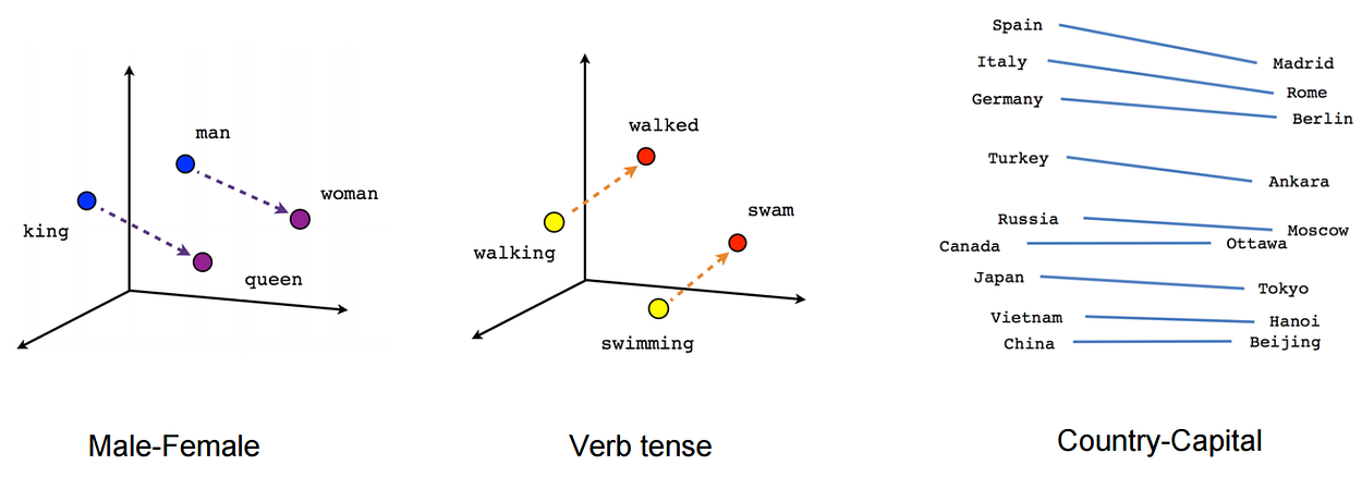
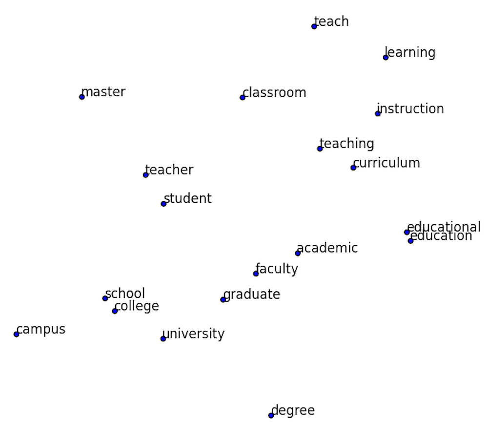
2. 訓練神經網路的過程中，每個嵌入的向量都會得到更新。如果你看到了部落格上面的圖片你就會發現在多維空間中詞與詞之間有多少相似性，這使我們能視覺化的瞭解詞語之間的關係，不僅僅是詞語，任何能通過嵌入層 Embedding 轉換成向量的內容都可以這樣做。

上面說的概念可能還有點含糊. 那我們就舉個栗子看看嵌入層 Embedding 對下面的句子做了什麼：）。Embedding的概念來自於word embeddings，如果您有興趣閱讀更多內容，可以查詢 word2vec 。

“deep learning is very deep”

使用嵌入層embedding 的第一步是通過索引對該句子進行編碼，這裡我們給每一個不同的句子分配一個索引，上面的句子就會變成這樣：

1 2 3 4 1

接下來會建立嵌入矩陣，我們要決定每一個索引需要分配多少個‘潛在因子’，這大體上意味著我們想要多長的向量，通常使用的情況是長度分配為32和50。在這篇部落格中，為了保持文章可讀性這裡為每個索引指定6個潛在因子。嵌入矩陣就會變成這樣：

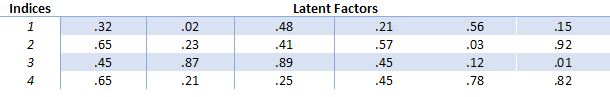
這樣，我們就可以使用嵌入矩陣來而不是龐大的one-hot編碼向量來保持每個向量更小。簡而言之，嵌入層embedding在這裡做的就是把單詞“deep”用向量[.32, .02, .48, .21, .56, .15]來表達。然而並不是每一個單詞都會被一個向量來代替，而是被替換為用於查詢嵌入矩陣中向量的索引。其次這種方法面對大資料時也可有效計算。由於在深度神經網路的訓練過程中嵌入向量也會被更新，我們就可以探索在高維空間中哪些詞語之間具有彼此相似性，再通過使用

Not Just Word Embeddings

These previous examples showed that word embeddings are very important in the world of Natural Language Processing. They allow us to capture relationships in language that are very difficult to capture otherwise. However, embedding layers can be used to embed many more things than just words. In my current research project I am using embedding layers to embed online user behavior. In this case I am assigning indices to user behavior like ‘page view on page type X on portal Y’ or ‘scrolled X pixels’. These indices are then used for constructing a sequence of user behavior.

In a comparison of ‘traditional’ machine learning models (SVM, Random Forest, Gradient Boosted Trees) with deep learning models (deep neural networks, recurrent neural networks) I found that this embedding approach worked very well for deep neural networks.

The ‘traditional’ machine learning models rely on a tabular input that is feature engineered. This means that we, as researchers, decide what gets turned into a feature. In these cases features could be: amount of homepages visited, amount of searches done, total amount of pixels scrolled. However, it is very difficult to capture the spatial (time) dimension when doing feature-engineering. By using deep learning and embedding layers we can efficiently capture this spatial dimension by supplying a sequence of user behavior (as indices) as input for the model.

In my research the Recurrent Neural Network with Gated Recurrent Unit/Long-Short Term Memory performed best. The results were very close. From the ‘traditional’ feature engineered models Gradient Boosted Trees performed best. I will write a blog post about this research in more detail in the future. I think my next blog post will explore Recurrent Neural Networks in more detail.

Other research has explored the use of embedding layers to encode student behavior in MOOCs (Piech et al., 2016) and users’ path through an online fashion store (Tamhane et al., 2017).

Recommender Systems

Embedding layers can even be used to deal with the sparse matrix problem in recommender systems. Since the deep learning course (fast.ai) uses recommender systems to introduce embedding layers I want to explore them here as well.

Recommender systems are being used everywhere and you are probably being influenced by them every day. The most common examples are Amazon’s product recommendation and Netflix’s program recommendation systems. Netflix actually held a $1,000,000 challenge to find the best collaborative filtering algorithm for their recommender system. You can see a visualization of one of these models here.

There are two main types of recommender systems and it is important to distinguish between the two.

1. Content-based filtering. This type of filtering is based on data about the item/product. For example, we have our users fill out a survey on what movies they like. If they say that they like sci-fi movies we recommend them sci-fi movies. In this case al lot of meta-information has to be available for all items.
2. Collaborative filtering: Let’s find other people like you, see what they liked and assume you like the same things. People like you = people who rated movies that you watched in a similar way. In a large dataset this has proven to work a lot better than the meta-data approach. Essentially asking people about their behavior is less good compared to looking at their actual behavior. Discussing this further is something for the psychologists among us.

In order to solve this problem we can create a huge matrix of the ratings of all users against all movies. However, in many cases this will create an extremely sparse matrix. Just think of your Netflix account. What percentage of their total supply of series and movies have you watched? It’s probably a pretty small percentage. Then, through gradient descent we can train a neural network to predict how high each user would rate each movie. Let me know if you would like to know more about the use of deep learning in recommender systems and we can explore it further together. In conclusion, embedding layers are amazing and should not be overlooked.

If you liked this posts be sure to recommend it so others can see it. You can also follow this profile to keep up with my process in the Fast AI course. See you there!

References

Piech, C., Bassen, J., Huang, J., Ganguli, S., Sahami, M., Guibas, L. J., & Sohl-Dickstein, J. (2015). Deep knowledge tracing. In Advances in Neural Information Processing Systems (pp. 505–513).

Tamhane, A., Arora, S., & Warrier, D. (2017, May). Modeling Contextual Changes in User Behaviour in Fashion e-Commerce. In Pacific-Asia Conference on Knowledge Discovery and Data Mining (pp. 539–550). Springer, Cham.

Embedding layers in keras

嵌入層embedding用在網路的開始層將你的輸入轉換成向量，所以當使用 Embedding前應首先判斷你的資料是否有必要轉換成向量。如果你有categorical資料或者資料僅僅包含整數（像一個字典一樣具有固定的數量）你可以嘗試下Embedding 層。
如果你的資料是多維的你可以對每個輸入共享嵌入層或嘗試單獨的嵌入層。

from keras.layers.embeddings import Embedding

Embedding(input_dim, output_dim, embeddings_initializer='uniform', embeddings_regularizer=None, activity_regularizer=None, embeddings_constraint=None, mask_zero=False, input_length=None)

-The first value of the Embedding constructor is the range of values in the input. In the example it’s 2 because we give a binary vector as input.
- The second value is the target dimension.
- The third is the length of the vectors we give.
- input_dim: int >= 0. Size of the vocabulary, ie. 1+maximum integer
index occuring in the input data.

How does embedding work? An example demonstrates best what is going on.

Assume you have a sparse vector [0,1,0,1,1,0,0] of dimension seven. You can turn it into a non-sparse 2d vector like so:

model = Sequential()
model.add(Embedding(2, 2, input_length=7))
model.compile('rmsprop', 'mse')
model.predict(np.array([[0,1,0,1,1,0,0]]))

array([[[ 0.03005414, -0.02224021],
        [ 0.03396987, -0.00576888],
        [ 0.03005414, -0.02224021],
        [ 0.03396987, -0.00576888],
        [ 0.03396987, -0.00576888],
        [ 0.03005414, -0.02224021],
        [ 0.03005414, -0.02224021]]], dtype=float32)

Where do these numbers come from? It’s a simple map from the given range to a 2d space:

model.layers[0].W.get_value()

array([[ 0.03005414, -0.02224021],
       [ 0.03396987, -0.00576888]], dtype=float32)

The 0-value is mapped to the first index and the 1-value to the second as can be seen by comparing the two arrays. The first value of the Embedding constructor is the range of values in the input. In the example it’s 2 because we give a binary vector as input. The second value is the target dimension. The third is the length of the vectors we give.
So, there is nothing magical in this, merely a mapping from integers to floats.

Now back to our ‘shining’ detection. The training data looks like a sequences of bits:

X

array([[ 0.,  1.,  1.,  1.,  0.,  1.,  0.,  1.,  0.,  0.,  0.,  0.,  0.,
         1.,  0.,  0.,  0.,  0.,  0.],
       [ 0.,  1.,  0.,  0.,  1.,  0.,  0.,  0.,  0.,  0.,  0.,  0.,  1.,
         0.,  0.,  0.,  0.,  0.,  0.],
       [ 0.,  1.,  1.,  0.,  0.,  0.,  0.,  0.,  0.,  0.,  0.,  1.,  0.,
         0.,  0.,  1.,  0.,  1.,  0.],
       [ 0.,  0.,  0.,  0.,  0.,  0.,  0.,  0.,  0.,  1.,  0.,  0.,  0.,
         0.,  1.,  0.,  1.,  0.,  0.],
       [ 0.,  0.,  0.,  0.,  0.,  0.,  1.,  0.,  1.,  0.,  1.,  0.,  0.,
         0.,  0.,  0.,  0.,  0.,  1.]])

If you want to use the embedding it means that the output of the embedding layer will have dimension (5, 19, 10). This works well with LSTM or GRU (see below) but if you want a binary classifier you need to flatten this to (5, 19*10):

model = Sequential()
model.add(Embedding(3, 10, input_length= X.shape[1] ))
model.add(Flatten())
model.add(Dense(1, activation='sigmoid'))
model.compile(loss='binary_crossentropy', optimizer='rmsprop')
model.fit(X, y=y, batch_size=200, nb_epoch=700, verbose=0, validation_split=0.2, show_accuracy=True, shuffle=True)

It detects ‘shining’ flawlessly:

model.predict(X)

array([[  1.00000000e+00],
       [  8.39483363e-08],
       [  9.71878720e-08],
       [  7.35597965e-08],
       [  9.91844118e-01]], dtype=float32)

An LSTM layer has historical memory and so the dimension outputted by the embedding works in this case, no need to flatten things:

model = Sequential()

model.add(Embedding(vocab_size, 10))
model.add(LSTM(5))
model.add(Dense(1, activation='sigmoid'))
model.compile(loss='binary_crossentropy', optimizer='rmsprop')
model.fit(X, y=y,  nb_epoch=500, verbose=0, validation_split=0.2, show_accuracy=True, shuffle=True)

Obviously, it predicts things as well:

model.predict(X)

array([[ 0.96855599],
       [ 0.01917232],
       [ 0.01917362],
       [ 0.01917258],
       [ 0.02341695]], dtype=float32)