貝葉斯分析——從數值積分到MCMC
阿新 • • 發佈:2019-01-08
Analytical solution
Numerical integration
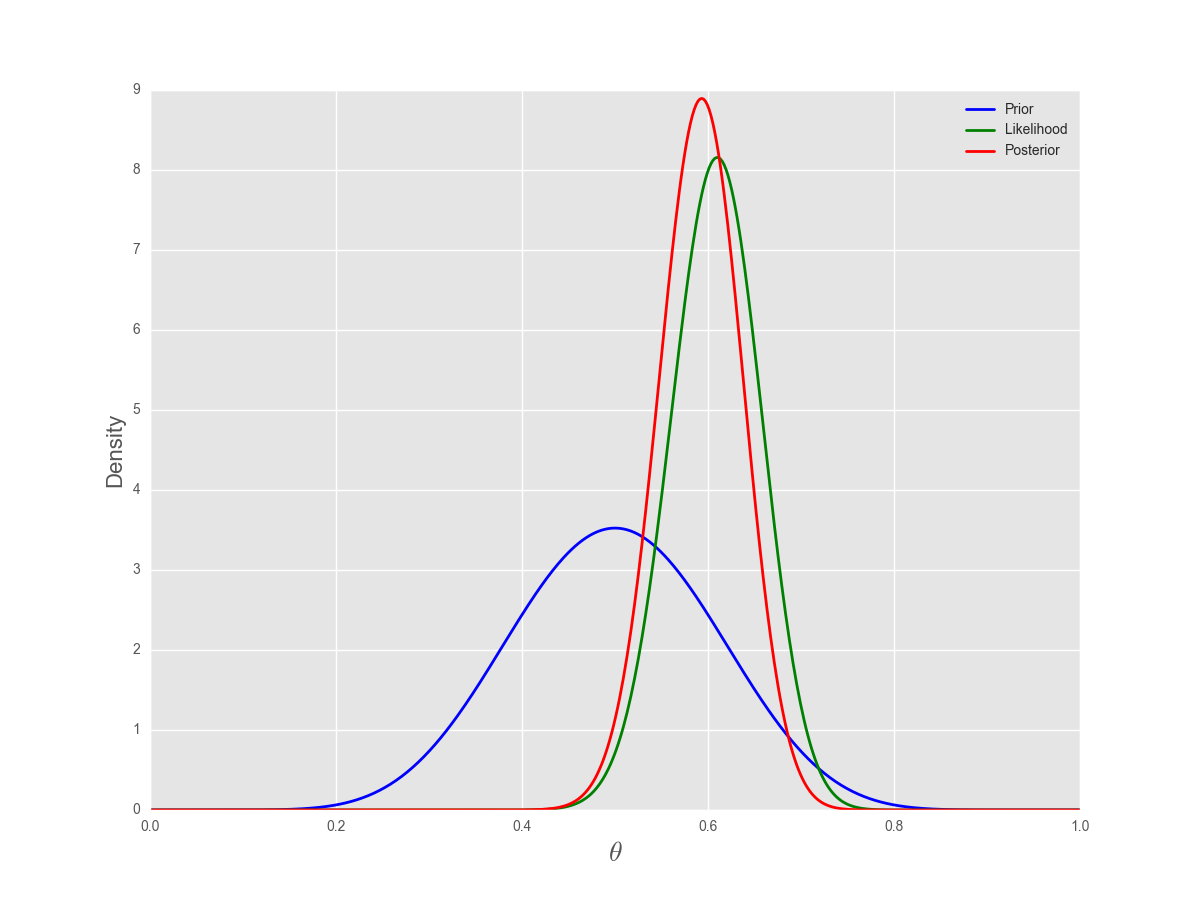
One simple way of numerical integration is to estimate the values on a grid of values for
One advantage of this is that the prior does not have to be conjugate (although the example below uses the same beta prior for ease of comaprsion), and so we are not restricted in our choice of an approproirate prior distribution. For example, the prior can be a mixture distribution
import numpy as np
import scipy.stats as st
import matplotlib.pyplot as plt

a, b = 10, 10
n, k = 100, 61

thetas = np.arange(0, 1, .001)
prior = st.beta(a, b)
poster = prior.pdf(thetas) * st.binom(n, thetas).pmf(k)
                    #
poster /= (poser.sum()/len(thetas))
                    # ∑p(θ)p(x|θ)
plt.plot(thetas, prior.pdf(thetas), 'b', lw=2, label='Prior')
plt.plot(thetas, n*st.binom(n, thetas).pmf(k), 'g', lw=2, label='Likelihood')
plt.plot(thetas, poster, 'r', lw=2, label='Posterior')

