
Matlab實現BP神經網路和RBF神經網路(一)
本實驗依託於教材《模式分類》第二版第六章(公式符號與書中一致)
實驗內容:
設計編寫BP神經網路和RBF神經網路,對給定資料集進行分類測試,並將分類準確率與SVM進行對比。
實驗環境:
matlab2016a
資料集:
資料集大小3*3000,表示3000個樣本,每個樣本包含2個特徵,第三行表示樣本所屬的分類。對於此次實驗編寫的BP神經網路和RBF神經網路,均將原始資料集分為訓練集和測試集兩部分,訓練集含2700個樣本,測試集300樣本,並且採用10-折交叉驗證,將資料集分為10份,每次將其中一份作為測試,剩餘作為訓練,總共進行10次驗證,得到10個準確率,將10個準確率求平均作為最終的衡量指標,與SVM分類效果進行對比。
BP網路和RBF網路相似但有所不同,因此分開闡述,先來設計BP網路。
BP神經網路:
BP網路有三層,輸入層,隱含層,輸出層,輸入層與隱含層之間有權值Wji,隱含層與輸出層之間有權值Wkj(i,j,k分別代表各層的神經元數目)。根據給定資料規模,可設計輸入層3個神經元(本來是2個神經元,加偏置後變為3),輸出層1個神經元,隱含層的神經元個數待會討論。
BP網路訓練演算法需要初始化以下引數:
(1)隱含層神經元個數
儘管輸入和輸出單元數分別由輸入向量的維數和類別數目決定,但隱單元個數並不簡單與此分類問題的外在特性相關。隱單元的個數決定了網路的表達能力,從而決定判決邊界的複雜度。對於較多的隱單元數,訓練誤差可變得很小,這是因為網路具有較高的表達能力,但這種場合下對測試樣本的誤差率會很高,是一個“過擬合”的例子;相反隱單元數過少,網路沒有足夠的自由度來擬合訓練集,同樣導致測試誤差高。一個簡單的規則經驗是選取隱單元的個數,使得網路的權值總數大致為n/10
(2)啟用函式
一般輸入層到隱含層的啟用函式需要非線性,飽和性和連續性,而隱含層到輸出層的啟用函式為線性即可。使用最多的啟用函式是sigmoid函式,具有下列形式的啟用函式可以很好的工作:
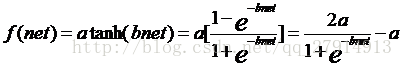
本次實驗中,取a=1.716,b=2/3,從而保證線性範圍為-1< net <+1。
(3)初始化權值
我們不能簡單將權值初始化為0,否則學習過程將不可能開始。我們要設定初始權值以獲得快速和均衡地學習,使所有權值同時達到最終的平衡值。為了使-1< net <+1,輸入權值應該選取

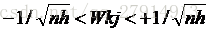 ,其中nh為隱含層的神經元個數。
(4)學習率eta和閾值theta
學習率決定網路收斂的速度,可以先設為0.1,如果學習速度過慢,則將學習率調大,如果準則函式在學習過程中發散,則將學習率調小。閾值決定訓練是否可以停止,設為0.01即可,根據實驗效果再調節。
相關引數初始化後,可以開始訓練,有三種訓練方式:隨機訓練、成批訓練和線上訓練。本實驗採用成批訓練,更新權值前所有樣本都提供一次,記為1個回合。
開始訓練前,記得增廣輸入向量,給輸入向量增加一維恆為1,作為偏置。資料訓練前可以先規範化,都對映到-1和1之間,經過實際測試,對於本資料,是否規範化對最後的準確率影響不大,但沒有規範化的資料收斂慢,執行時間長。
實驗程式碼:
(1)函式 Batch_BP_neutral_network.m(建議使用matlab檢視)
function correct_rate=Batch_BP_Neural_Network(train_data,test_data,hidden_layers,Wji,Wkj,theta,eta)
%-------------------------------------------------------------------
%Batch back-propagation neural network function which includes input layer(multiple layers with bias)、
%hidden layer(multiple layers) and output(one layer)
%Inputs:
%train_data     -train data(including samples and its target output)
%test_data      -test data(including samples and its target output)
%hidden_layers  -numbers of hidden layers
%Wji            -weights between input layer and hidden layer
%Wkj            -weights between hidden layer and putput layer
%theta          -threhold of target function
%eta            -learnning rate
%Output:
%correct_rate:  -classification correct rate of the test data
%-------------------------------------------------------------------
[rows,cols]=size(train_data);
train_input=train_data(1:rows-1,:);
train_target=train_data(rows,:);
test_input=test_data(1:rows-1,:);
test_target=test_data(rows,:);
%augmentation the train and test input
train_bias=ones(1,cols);
test_bias=ones(1,size(test_data,2));
train_input=[train_bias;train_input];
test_input=[test_bias;test_input];
%batch bp algorithm
r=0;   %initialize the episode
J=zeros(1,1000); %initialize the error function
while(1)     %outer loop
    r=r+1;m=0;DELTA_Wji=zeros(hidden_layers,rows);DELTA_Wkj=zeros(1,hidden_layers);  %initialization
    while(1)    %inner loop
        m=m+1;
        netj=zeros(1,hidden_layers);
        yj=zeros(1,hidden_layers);
        for j=1:hidden_layers
            netj(1,j)=sum(train_input(:,m)'.*Wji(j,:));   %sum of product
            yj(1,j)=3.432/(1+exp(-2*netj(1,j)/3))-1.716;   %activation
        end
        netk=sum(yj(1,:).*Wkj(1,:));  %sum of product,output layer has only one neutron
        zk=netk;   %activation
        J(1,r)=J(1,r)+(train_target(1,m)-zk)^2/2;   %every sample has a error
        for j=1:hidden_layers
            delta_k=(train_target(1,m)-zk);  %the sensitivity of output neutrons
            DELTA_Wkj(1,j)=DELTA_Wkj(1,j)+eta*delta_k*yj(1,j); %update the DELTA_Wkj
        end
        delta_j=zeros(1,hidden_layers);
        for j=1:hidden_layers
            delta_j(1,j)=Wkj(1,j)*delta_k*(2.288*exp(-2*netj(1,j)/3)/(1+exp(-2*netj(1,j)/3)^2)); %the sensitivity of hidden neutrons
            for i=1:rows
                DELTA_Wji(j,i)=DELTA_Wji(j,i)+eta*delta_j(1,j)*train_input(i,m);   %update the DELTA_Wji
            end
        end
        if(m==cols)  %all samples has been trained(one episode)
            break;   %back to outer loop
        end
    end    %end inner loop
    for j=1:hidden_layers
        Wkj(1,j)=Wkj(1,j)+DELTA_Wkj(1,j);   %update Wkj
    end
    for j=1:hidden_layers
        for i=1:rows
            Wji(j,i)=Wji(j,i)+DELTA_Wji(j,i);   %update Wji
        end
    end
    J(1,r)=J(1,r)/cols;
    if((r>=2)&&abs(J(1,r)-J(1,r-1))<theta)  %determine when to stop
        %disp('ok!');disp(r);
        %plot(0:r-1,J(1,1:r));hold on;
        %start to test the model
        correct=0;
        for i=1:size(test_data,2)
            test_netj=zeros(1,hidden_layers);
            test_yj=zeros(1,hidden_layers);
            for j=1:hidden_layers
                test_netj(1,j)=sum(test_input(:,i)'.*Wji(j,:));   %sum of product
                test_yj(1,j)=3.432/(1+exp(-2*test_netj(1,j)/3))-1.716;   %activation
            end
            test_netk=sum(test_yj(1,:).*Wkj(1,:));  %sum of product,output layer has only one neutron
            test_zk=test_netk;   %activation
            if((test_zk>0&&test_target(1,i)==1)||(test_zk<0&&test_target(1,i)==-1))
                correct=correct+1;
            end
        end
        correct_rate=correct/size(test_data,2);
        break;
    end
end
(2)主函式
clear;
load sample_ex6.mat;  %load data
[M,N]=size(data);
hidden_layers=10;
theta=0.001;
eta=0.00001;
wkj=-1/(hidden_layers^0.5)+2/(hidden_layers^0.5)*rand(1,hidden_layers);
wji=-1/(M^0.5)+2/(M^0.5)*rand(hidden_layers,M);
%input data normalization
[norm_data,norm_dataps]=mapminmax(data);
%10-fold crossing validation
sub_N=N/10;
rates=zeros(1,10);
for i=1:10
    norm_testdata=data(:,1:sub_N);  %set the first part as testdata
    norm_traindata=data(:,sub_N+1:N);   %set the next nine part as traindata
    rates(1,i)=Batch_BP_Neural_Network(norm_traindata,norm_testdata,hidden_layers,wji,wkj,theta,eta);
    data=[norm_traindata,norm_testdata];
end
disp('the accuracy of ten validation:')
disp(rates);disp('the average accuracy is:')
ave_rate=sum(rates)/10;
disp(ave_rate);
實驗結果:
訓練完後,輸入測試資料求出分類的準確率,由於採取的是10-fold交叉驗證,需要訓練10次,下圖顯示10次訓練誤差函式與回合的曲線:
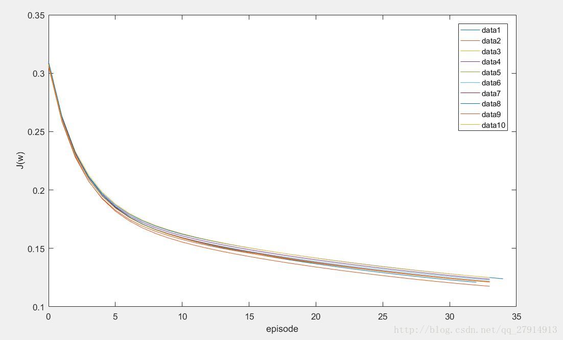
可以看出,隨著訓練的進行,誤差函式一直減小,直到前後兩次誤差函式的差小於閾值停止訓練。
每次測試的準確率以及最後的平均準確率如下圖:
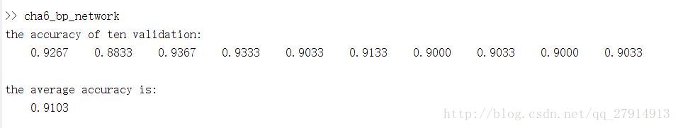
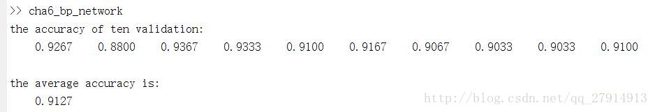
經過多次實驗,平均準確率都在91%左右,不是很高,為什麼說不是很高,看後面與SVM的對比就知道了。並且發現隱含層神經元個數取62或者10結果都差不多,準確率相差不大。但隱單元個數少執行時間短,10次交叉驗證的總時間為:
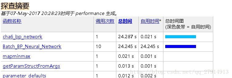
每次執行時間均有差異,十幾秒到二十幾秒之間。
這是BP網路設計部分,RBF網路設計以及與SVM的對比 將在下一篇博文:Matlab實現BP神經網路和RBF神經網路(二)中討論。