
SSD演算法Tensorflow版詳解(一)
之前看了SSD的論文,但也只是僅僅停留在論文層面,這幾天在github上找到了一位大神在一年前用Tensorflow實現了SSD演算法。這幾天也抽空閱讀了下程式碼,主要分析了下幾個重要的模組,接下來做一個簡單的總結。
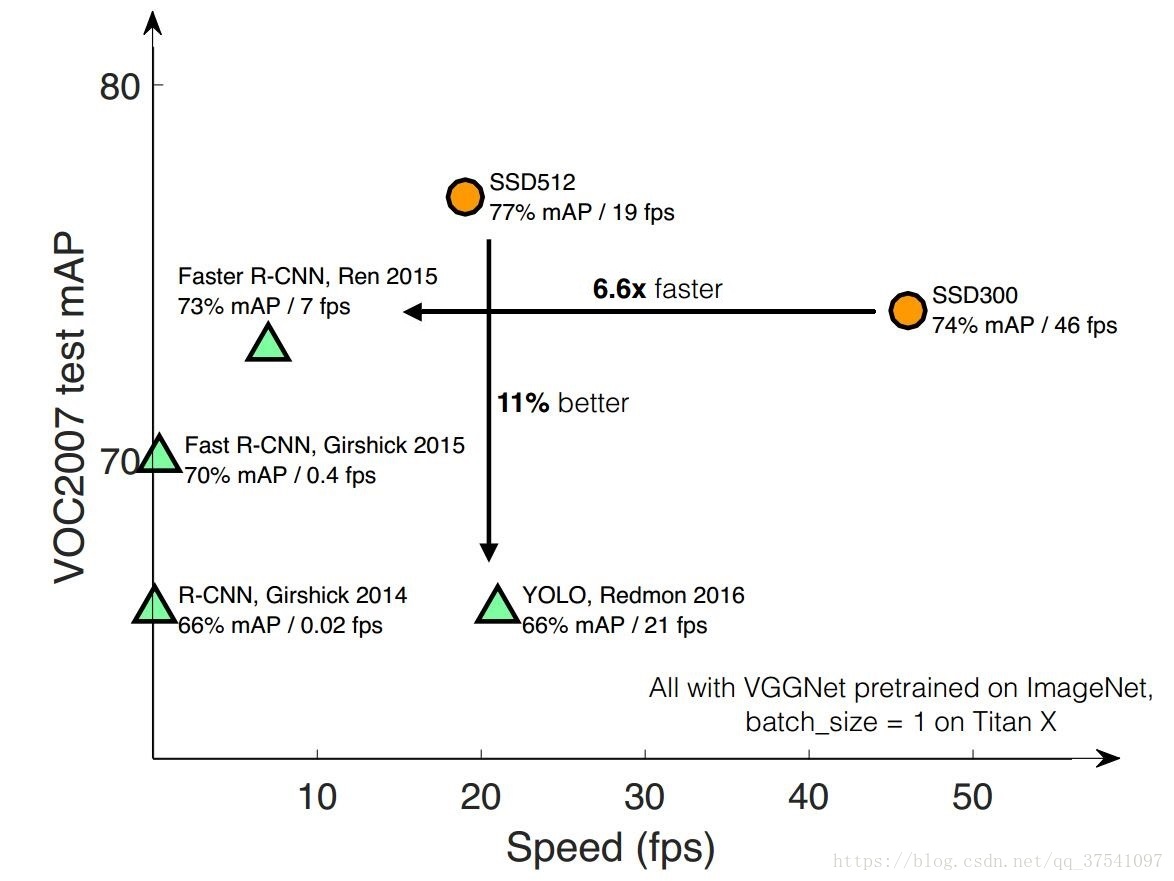
SSD(Single Shot MultiBox Detector)是大神Wei Liu在 ECCV 2016上發表的一種的目標檢測演算法。對於輸入影象大小300x300的版本在VOC2007資料集上達到了72.1%mAP的準確率並且檢測速度達到了驚人的58FPS( Faster RCNN:73.2%mAP,7FPS; YOLOv1: 63.4%mAP,45FPS ),500x500的版本達到了75.1%mAP的準確率。當然演算法YOLOv2已經趕上了SSD,YOLOv3已經超越SSD,但SSD演算法依舊值得研究。
首先放出Tensorflow版的SSD程式碼,連結。
接下來,通過5個方面(SSD重要引數設定、SSD網路結構、預設框(default box)的生成、預設框與GT的匹配以及偏差計算、Loss函式計算)來分析ssd300x300版本的程式碼。
SSD重要引數設定
在ssd_vgg_300.py檔案中初始化重要的網路引數,主要有用於生成預設框的特徵層,每層預設框的預設尺寸以及長寬比例:default_params = SSDParams( img_shape=(300, 300), # 圖片輸入尺寸 num_classes=21, # 預測類別20+1(背景) no_annotation_label=21, feat_layers=['block4', 'block7', 'block8', 'block9', 'block10', 'block11'], # 用於生成default box的特徵層 feat_shapes=[(38, 38), (19, 19), (10, 10), (5, 5), (3, 3), (1, 1)], # 對應特徵層的特徵圖尺寸 anchor_size_bounds=[0.15, 0.90], # Smin = 0.15, Smax = 0.9 # anchor_size_bounds=[0.20, 0.90], anchor_sizes=[(21., 45.), # 當前層與下一層的預測預設矩形邊框尺寸,即Sk的值,與論文中的計算公式並不對應 (45., 99.), (99., 153.), (153., 207.), (207., 261.), (261., 315.)], anchor_ratios=[[2, .5], # 生成預設框的形狀比例,不包含1:1的比例 [2, .5, 3, 1./3], [2, .5, 3, 1./3], [2, .5, 3, 1./3], [2, .5], [2, .5]], anchor_steps=[8, 16, 32, 64, 100, 300], # 特徵圖上一步對應在原圖上的跨度 anchor_step*feat_shapey與等於300 anchor_offset=0.5, # 偏移 normalizations=[20, -1, -1, -1, -1, -1], # 特徵層是否正則處理 prior_scaling=[0.1, 0.1, 0.2, 0.2] # 預設框與真實框的差異縮放比例 )
除了以上引數需要注意外,還要留意下各個種類及其對應的Label
在pascalvoc_common.py檔案中給出了相應資訊,注意0代表著背景的概率。
VOC_LABELS = {
    'none': (0, 'Background'),
    'aeroplane': (1, 'Vehicle'),
    'bicycle': (2, 'Vehicle'),
    'bird': (3, 'Animal'),
    'boat': (4, 'Vehicle'),
    'bottle': (5, 'Indoor'),
    'bus': (6, 'Vehicle'),
    'car': (7, 'Vehicle'),
    'cat': (8, 'Animal'),
    'chair': (9, 'Indoor'),
    'cow': (10, 'Animal'),
    'diningtable': (11, 'Indoor'),
    'dog': (12, 'Animal'),
    'horse': (13, 'Animal'),
    'motorbike': (14, 'Vehicle'),
    'person': (15, 'Person'),
    'pottedplant': (16, 'Indoor'),
    'sheep': (17, 'Animal'),
    'sofa': (18, 'Indoor'),
    'train': (19, 'Vehicle'),
    'tvmonitor': (20, 'Indoor'),
}
SSD網路結構

在程式碼中作者主要利用了Tensorflow的Slim框架搭建的網路。
# 建立SSD網路
def ssd_net(inputs,
            num_classes=SSDNet.default_params.num_classes,
            feat_layers=SSDNet.default_params.feat_layers,
            anchor_sizes=SSDNet.default_params.anchor_sizes,
            anchor_ratios=SSDNet.default_params.anchor_ratios,
            normalizations=SSDNet.default_params.normalizations,
            is_training=True,
            dropout_keep_prob=0.5,
            prediction_fn=slim.softmax,
            reuse=None,
            scope='ssd_300_vgg'):
    """SSD net definition.
    """
    # if data_format == 'NCHW':
    #     inputs = tf.transpose(inputs, perm=(0, 3, 1, 2))

    # End_points collect relevant activations for external use.
    # 用於收集每一層的輸出
    end_points = {}
    with tf.variable_scope(scope, 'ssd_300_vgg', [inputs], reuse=reuse):
        # Original VGG-16 blocks.
        net = slim.repeat(inputs, 2, slim.conv2d, 64, [3, 3], scope='conv1')
        end_points['block1'] = net
        net = slim.max_pool2d(net, [2, 2], scope='pool1')
        # Block 2.
        net = slim.repeat(net, 2, slim.conv2d, 128, [3, 3], scope='conv2')
        end_points['block2'] = net
        net = slim.max_pool2d(net, [2, 2], scope='pool2')
        # Block 3.
        net = slim.repeat(net, 3, slim.conv2d, 256, [3, 3], scope='conv3')
        end_points['block3'] = net
        net = slim.max_pool2d(net, [2, 2], scope='pool3')
        # Block 4.
        net = slim.repeat(net, 3, slim.conv2d, 512, [3, 3], scope='conv4')
        end_points['block4'] = net
        net = slim.max_pool2d(net, [2, 2], scope='pool4')
        # Block 5.
        net = slim.repeat(net, 3, slim.conv2d, 512, [3, 3], scope='conv5')
        end_points['block5'] = net
        net = slim.max_pool2d(net, [3, 3], stride=1, scope='pool5')

        # Additional SSD blocks.
        # Block 6: let's dilate the hell out of it!
        net = slim.conv2d(net, 1024, [3, 3], rate=6, scope='conv6')
        end_points['block6'] = net
        net = tf.layers.dropout(net, rate=dropout_keep_prob, training=is_training)
        # Block 7: 1x1 conv. Because the fuck.
        net = slim.conv2d(net, 1024, [1, 1], scope='conv7')
        end_points['block7'] = net
        net = tf.layers.dropout(net, rate=dropout_keep_prob, training=is_training)

        # Block 8/9/10/11: 1x1 and 3x3 convolutions stride 2 (except lasts).
        end_point = 'block8'
        with tf.variable_scope(end_point):
            net = slim.conv2d(net, 256, [1, 1], scope='conv1x1')
            net = custom_layers.pad2d(net, pad=(1, 1))
            net = slim.conv2d(net, 512, [3, 3], stride=2, scope='conv3x3', padding='VALID')
        end_points[end_point] = net
        end_point = 'block9'
        with tf.variable_scope(end_point):
            net = slim.conv2d(net, 128, [1, 1], scope='conv1x1')
            net = custom_layers.pad2d(net, pad=(1, 1))
            net = slim.conv2d(net, 256, [3, 3], stride=2, scope='conv3x3', padding='VALID')
        end_points[end_point] = net
        end_point = 'block10'
        with tf.variable_scope(end_point):
            net = slim.conv2d(net, 128, [1, 1], scope='conv1x1')
            net = slim.conv2d(net, 256, [3, 3], scope='conv3x3', padding='VALID')
        end_points[end_point] = net
        end_point = 'block11'
        with tf.variable_scope(end_point):
            net = slim.conv2d(net, 128, [1, 1], scope='conv1x1')
            net = slim.conv2d(net, 256, [3, 3], scope='conv3x3', padding='VALID')
        end_points[end_point] = net

        # Prediction and localisations layers.
        # 預測類別和位置調整
        predictions = []
        logits = []
        localisations = []
        for i, layer in enumerate(feat_layers):
            with tf.variable_scope(layer + '_box'):
                # 接受特徵層的輸出,生成類別和位置預測
                p, l = ssd_multibox_layer(end_points[layer],
                                          num_classes,
                                          anchor_sizes[i],
                                          anchor_ratios[i],
                                          normalizations[i])
            # 收集每一層的預測結果
            predictions.append(prediction_fn(p))  # prediction_fc為softmax函式,預測類別
            logits.append(p)  # 概率
            localisations.append(l)  # 預測位置偏移

        return predictions, localisations, logits, end_points
網路結構的搭建比較簡單,這裡在簡單分析下接在每個用於預測的特徵層後的卷積層(用於生成預設框對應目標類別以及中心點偏移量和長寬調整比例),ssd_multibox_layer函式:
def ssd_multibox_layer(inputs,  # 輸入的特徵層
                       num_classes,
                       sizes,  # 當前層與下一層的預測預設矩形邊框尺寸,即Sk的值
                       ratios=[1],  # 矩形框長寬比
                       normalization=-1,  # 是否正則化
                       bn_normalization=False):
    """Construct a multibox layer, return a class and localization predictions.
    生成預測中心偏移量和寬高調整比例
    """
    net = inputs
    if normalization > 0:
        net = custom_layers.l2_normalization(net, scaling=True)
    # Number of anchors.
    num_anchors = len(sizes) + len(ratios)

    # Location.預設框位置偏移量預測
    num_loc_pred = num_anchors * 4
    loc_pred = slim.conv2d(net, num_loc_pred, [3, 3], activation_fn=None,
                           scope='conv_loc')
    loc_pred = custom_layers.channel_to_last(loc_pred)
    loc_pred = tf.reshape(loc_pred,
                          tensor_shape(loc_pred, 4)[:-1]+[num_anchors, 4])
    # Class prediction.預設框內目標類別預測
    num_cls_pred = num_anchors * num_classes
    cls_pred = slim.conv2d(net, num_cls_pred, [3, 3], activation_fn=None,
                           scope='conv_cls')
    cls_pred = custom_layers.channel_to_last(cls_pred)
    cls_pred = tf.reshape(cls_pred,
                          tensor_shape(cls_pred, 4)[:-1]+[num_anchors, num_classes])
    return cls_pred, loc_pred
預設框(default box)的生成
對與每個用來預測的特徵圖,按照不同的大小(scale)和長寬比(ratio)生成k個預設框(default box),k的值由scale和ratio共同決定。例如對於特徵層'block4',特徵圖尺寸為38x38,預設框size為(21., 45.)(注意45是下一特徵層預設框的大小),預設框ratio為(2., 0.5),故k=4(尺寸21的有1:1, 1:2, 2:1三個預設框,以及論文中額外新增的一個尺寸為sqrt(21, 45)的1:1一個預設框),該層總共會生成38x38x4個預設框。
對於預設框的大小論文由給出計算公式:
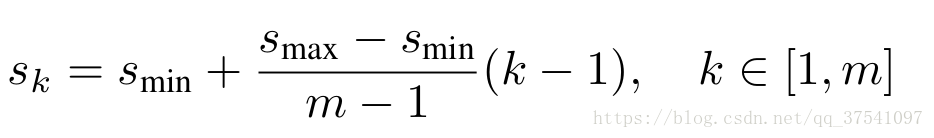
Smin論文中為0.2程式碼中為1.5, Smax論文中程式碼中都為0.9。m是用於預測的特徵圖個數,k代表層數。但程式碼中每層預設框大小並不與計算公式對應。
# 生成一層anchor box
def ssd_anchor_one_layer(img_shape,  # 原始影象shape
                         feat_shape,  # 特徵圖shape
                         sizes,  # 預設box大小
                         ratios,  # 預設box長寬比
                         step,  # 特徵圖上一步對應在原圖上的跨度
                         offset=0.5,
                         dtype=np.float32):
    """Computer SSD default anchor boxes for one feature layer.

    Determine the relative position grid of the centers, and the relative
    width and height.

    Arguments:
      feat_shape: Feature shape, used for computing relative position grids;
      size: Absolute reference sizes;
      ratios: Ratios to use on these features;
      img_shape: Image shape, used for computing height, width relatively to the
        former;
      offset: Grid offset.

    Return:
      y, x, h, w: Relative x and y grids, and height and width.
    """
    # Compute the position grid: simple way.
    # y, x = np.mgrid[0:feat_shape[0], 0:feat_shape[1]]
    # y = (y.astype(dtype) + offset) / feat_shape[0]
    # x = (x.astype(dtype) + offset) / feat_shape[1]
    # Weird SSD-Caffe computation using steps values...
    # 計算預設框中心座標(相對原圖)
    y, x = np.mgrid[0:feat_shape[0], 0:feat_shape[1]]
    y = (y.astype(dtype) + offset) * step / img_shape[0]
    x = (x.astype(dtype) + offset) * step / img_shape[1]

    # Expand dims to support easy broadcasting.
    y = np.expand_dims(y, axis=-1)
    x = np.expand_dims(x, axis=-1)

    # Compute relative height and width.
    # Tries to follow the original implementation of SSD for the order.
    num_anchors = len(sizes) + len(ratios)  # 預設框的個數
    h = np.zeros((num_anchors, ), dtype=dtype)  # 初始化高
    w = np.zeros((num_anchors, ), dtype=dtype)  # 初始化寬
    # Add first anchor boxes with ratio=1.
    h[0] = sizes[0] / img_shape[0]  # 新增長寬比為1的預設框
    w[0] = sizes[0] / img_shape[1]
    di = 1
    if len(sizes) > 1:
        h[1] = math.sqrt(sizes[0] * sizes[1]) / img_shape[0]  # 新增一組特殊的預設框,長寬比為1,大小為sqrt(s(i) + s(i+1))
        w[1] = math.sqrt(sizes[0] * sizes[1]) / img_shape[1]
        di += 1
    for i, r in enumerate(ratios):  # 新增不同比例的預設框(ratios中不含1)
        h[i+di] = sizes[0] / img_shape[0] / math.sqrt(r)
        w[i+di] = sizes[0] / img_shape[1] * math.sqrt(r)
    return y, x, h, w
預設框與GT的匹配、以及偏差計算
該部分主要是預設框的匹配策略(和原論文中的Matching strategy有些不同,該部分僅僅是尋找與之IOU最大的GTbox,並沒有通過閾值0.5去篩選正樣本),將每個預設框與ground truth box進行匹配,尋找與之IOU(交併比)最大的ground truth box,並計算每個預設框與之匹配的ground truth box的偏差(矩形框中心座標x、y方向偏移量,以及高h寬w的縮放比例)。
根據程式的執行流程首先是ssd_vgg_300.py檔案中的bboxes_encode函式:
    def bboxes_encode(self, labels, bboxes, anchors,  # lables是GT box對應的標籤, bboxes是GT box對應的座標資訊
                      scope=None):                    # anchors是生成的預設框
        """Encode labels and bounding boxes.
        """
        return ssd_common.tf_ssd_bboxes_encode(
            labels, bboxes, anchors,
            self.params.num_classes,
            self.params.no_annotation_label,
            ignore_threshold=0.5,
            prior_scaling=self.params.prior_scaling,
            scope=scope)
接下來我們在分析bboxes_encode函式中的tf_ssd_bboxes_encode函式(位於ssd_common.py檔案中):
def tf_ssd_bboxes_encode(labels,  # 真實標籤
                         bboxes,  # 真實bbox
                         anchors,  # 存放每一個預測層生成的預設框
                         num_classes,
                         no_annotation_label,
                         ignore_threshold=0.5,
                         prior_scaling=[0.1, 0.1, 0.2, 0.2],
                         dtype=tf.float32,
                         scope='ssd_bboxes_encode'):
    """Encode groundtruth labels and bounding boxes using SSD net anchors.
    Encoding boxes for all feature layers.

    Arguments:
      labels: 1D Tensor(int64) containing groundtruth labels;
      bboxes: Nx4 Tensor(float) with bboxes relative coordinates;
      anchors: List of Numpy array with layer anchors;
      matching_threshold: Threshold for positive match with groundtruth bboxes;
      prior_scaling: Scaling of encoded coordinates.

    Return:
      (target_labels, target_localizations, target_scores):
        Each element is a list of target Tensors.
    """
    with tf.name_scope(scope):
        target_labels = []  # 存放匹配到的GTbox的label的容器
        target_localizations = []  # 存放匹配到的GTbox的位置資訊的容器
        target_scores = []  # 存放預設框與匹配到的GTbox的IOU(交併比)
        for i, anchors_layer in enumerate(anchors):  # 遍歷每個預測層的預設框
            with tf.name_scope('bboxes_encode_block_%i' % i):
                t_labels, t_loc, t_scores = \
                    tf_ssd_bboxes_encode_layer(labels, bboxes, anchors_layer,  # 匹配預設框的ground truth box並計算偏差
                                               num_classes, no_annotation_label,
                                               ignore_threshold,
                                               prior_scaling, dtype)
                target_labels.append(t_labels)  # 匹配到的ground truth box對應標籤
                target_localizations.append(t_loc)  # 預設框與匹配到的ground truth box的座標差異
                target_scores.append(t_scores)  # 預設框與匹配到的ground truth box的IOU(交併比)
return target_labels, target_localizations, target_scores在tf_ssd_bboxes_encode函式中最主要的就是tf_ssd_bboxes_encode_layer函式(需要注意的是:在該函式中僅僅只是尋找與每個預設框最匹配的GTbox,並沒有進行篩選正負樣本,關於正負樣本的選取會在下一部分losses計算中講述),接下來我們在仔細分析該函式:
def tf_ssd_bboxes_encode_layer(labels,  # GTbox類別
                               bboxes,  # GTbox的位置資訊
                               anchors_layer,  # 預設框座標資訊(中心點座標以及寬、高)
                               num_classes,
                               no_annotation_label,
                               ignore_threshold=0.5,
                               prior_scaling=[0.1, 0.1, 0.2, 0.2],
                               dtype=tf.float32):
    """Encode groundtruth labels and bounding boxes using SSD anchors from
    one layer.

    Arguments:
      labels: 1D Tensor(int64) containing groundtruth labels;
      bboxes: Nx4 Tensor(float) with bboxes relative coordinates;
      anchors_layer: Numpy array with layer anchors;
      matching_threshold: Threshold for positive match with groundtruth bboxes;
      prior_scaling: Scaling of encoded coordinates.

    Return:
      (target_labels, target_localizations, target_scores): Target Tensors.
    """
    # Anchors coordinates and volume.
    yref, xref, href, wref = anchors_layer
    ymin = yref - href / 2.  # 轉換到預設框的左上角座標以及右下角座標
    xmin = xref - wref / 2.
    ymax = yref + href / 2.
    xmax = xref + wref / 2.
    vol_anchors = (xmax - xmin) * (ymax - ymin)  # 預設框的面積

    # Initialize tensors...
    # 初始化各引數
    shape = (yref.shape[0], yref.shape[1], href.size)
    feat_labels = tf.zeros(shape, dtype=tf.int64)  # 存放預設框匹配的GTbox標籤
    feat_scores = tf.zeros(shape, dtype=dtype)  # 存放預設框與匹配的GTbox的IOU(交併比)

    feat_ymin = tf.zeros(shape, dtype=dtype)  # 存放預設框匹配到的GTbox的座標資訊
    feat_xmin = tf.zeros(shape, dtype=dtype)
    feat_ymax = tf.ones(shape, dtype=dtype)
    feat_xmax = tf.ones(shape, dtype=dtype)

    def jaccard_with_anchors(bbox):  # 計算重疊度函式
        """Compute jaccard score between a box and the anchors.
        """
        int_ymin = tf.maximum(ymin, bbox[0])
        int_xmin = tf.maximum(xmin, bbox[1])
        int_ymax = tf.minimum(ymax, bbox[2])
        int_xmax = tf.minimum(xmax, bbox[3])
        h = tf.maximum(int_ymax - int_ymin, 0.)
        w = tf.maximum(int_xmax - int_xmin, 0.)
        # Volumes.
        inter_vol = h * w
        union_vol = vol_anchors - inter_vol \
            + (bbox[2] - bbox[0]) * (bbox[3] - bbox[1])
        jaccard = tf.div(inter_vol, union_vol)
        return jaccard

    def intersection_with_anchors(bbox):
        """Compute intersection between score a box and the anchors.
        """
        int_ymin = tf.maximum(ymin, bbox[0])
        int_xmin = tf.maximum(xmin, bbox[1])
        int_ymax = tf.minimum(ymax, bbox[2])
        int_xmax = tf.minimum(xmax, bbox[3])
        h = tf.maximum(int_ymax - int_ymin, 0.)
        w = tf.maximum(int_xmax - int_xmin, 0.)
        inter_vol = h * w
        scores = tf.div(inter_vol, vol_anchors)
        return scores

    def condition(i, feat_labels, feat_scores,  # 迴圈條件
                  feat_ymin, feat_xmin, feat_ymax, feat_xmax):
        """Condition: check label index.
        """
        r = tf.less(i, tf.shape(labels))  # tf.shape(labels)GTbox的個數,當i<=tf.shape(labels)是返回True
        return r[0]

    def body(i, feat_labels, feat_scores,  # 迴圈執行主體
             feat_ymin, feat_xmin, feat_ymax, feat_xmax):
        """Body: update feature labels, scores and bboxes.
        Follow the original SSD paper for that purpose:
          - assign values when jaccard > 0.5;
          - only update if beat the score of other bboxes.
        尋找該層所有預設框匹配滿足條件的GTbox
        """
        # Jaccard score.
        label = labels[i]
        bbox = bboxes[i]
        jaccard = jaccard_with_anchors(bbox)   # 計算該層所有的預設框與該真實框的交併比
        # Mask: check threshold + scores + no annotations + num_classes.
        mask = tf.greater(jaccard, feat_scores)  # 交併比是否比之前匹配的GTbox大
        # mask = tf.logical_and(mask, tf.greater(jaccard, matching_threshold))
        mask = tf.logical_and(mask, feat_scores > -0.5)  # 暫不清楚意義,但這裡並不是為了獲取正樣本所以並不是大於0.5
        mask = tf.logical_and(mask, label < num_classes)  # 感覺沒有任何意義真實標籤label肯定小於num_classes,防止出錯?
        imask = tf.cast(mask, tf.int64)  # 轉型
        fmask = tf.cast(mask, dtype)  # dtype float32
        # Update values using mask. 根據mask更新標籤和交併比
        feat_labels = imask * label + (1 - imask) * feat_labels  # 當imask為1時更新標籤
        feat_scores = tf.where(mask, jaccard, feat_scores)  # 當mask為true時更新為jaccard,否則為feat_score

        feat_ymin = fmask * bbox[0] + (1 - fmask) * feat_ymin  # 當fmask為1.0時更新座標資訊
        feat_xmin = fmask * bbox[1] + (1 - fmask) * feat_xmin
        feat_ymax = fmask * bbox[2] + (1 - fmask) * feat_ymax
        feat_xmax = fmask * bbox[3] + (1 - fmask) * feat_xmax

        # Check no annotation label: ignore these anchors...
        # interscts = intersection_with_anchors(bbox)
        # mask = tf.logical_and(interscts > ignore_threshold,
        #                       label == no_annotation_label)
        # # Replace scores by -1.
        # feat_scores = tf.where(mask, -tf.cast(mask, dtype), feat_scores)

        return [i+1, feat_labels, feat_scores,
                feat_ymin, feat_xmin, feat_ymax, feat_xmax]
    # Main loop definition.
    i = 0
    [i, feat_labels, feat_scores,
     feat_ymin, feat_xmin,
     feat_ymax, feat_xmax] = tf.while_loop(condition, body,  # tf.while_loop是一個迴圈函式condition是迴圈條件,body是迴圈體
                                           [i, feat_labels, feat_scores,   # 第三項是引數
                                            feat_ymin, feat_xmin,
                                            feat_ymax, feat_xmax])
    # Transform to center / size. 轉換回中心座標以及寬高
    feat_cy = (feat_ymax + feat_ymin) / 2.
    feat_cx = (feat_xmax + feat_xmin) / 2.
    feat_h = feat_ymax - feat_ymin
    feat_w = feat_xmax - feat_xmin
    # Encode features.
    feat_cy = (feat_cy - yref) / href / prior_scaling[0]  # 預設框中心與匹配的真實框中心座標偏差
    feat_cx = (feat_cx - xref) / wref / prior_scaling[1]
    feat_h = tf.log(feat_h / href) / prior_scaling[2]  # 高和寬的偏差
    feat_w = tf.log(feat_w / wref) / prior_scaling[3]
    # Use SSD ordering: x / y / w / h instead of ours.
    feat_localizations = tf.stack([feat_cx, feat_cy, feat_w, feat_h], axis=-1)
    return feat_labels, feat_localizations, feat_scores
Loss函式計算
SSD的Loss函式包含兩項:(1)預測類別損失(2)預測位置偏移量損失:
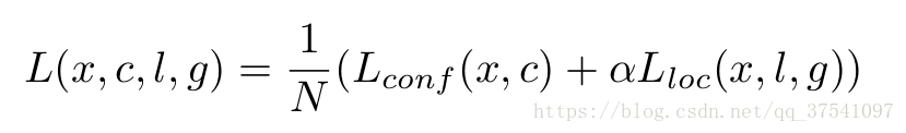
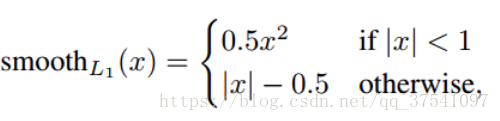
Loss中的N代表著被挑選出來的預設框個數(包括正樣本和負樣本),L(los)即位置偏移量損失是Smooth L1 loss(是預設框與GTbox之間的位置偏移與網路預測出的位置偏移量之間的損失),L(conf)即預測類別損失是多類別softmax loss,α的值設定為1. Smooth L1 loss定義為:
L(los)損失函式的定義為:
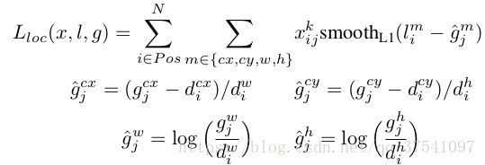
根據函式定義我們可以看到L(los)損失函式主要有四部分:中心座標cx的偏移量損失,中心點座標cy的偏移損失,寬度w的縮放損失以及高度h的縮放損失。式中的l表示的是預測的座標偏移量,g表示的是預設框與之匹配的GTbox的座標偏移量。
L(conf)多類別softmax loss損失定義為:
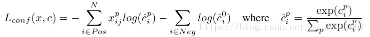
根據函式定義我們可以看到L(conf)損失由兩部分組成:正樣本(Pos)損失和負樣本(Neg)損失。

接下來我們來分析下ssd_vgg_300.py檔案中的ssd_losses函式,需要注意的是負樣本的選取(論文中Hard negative mining部分),什麼是hard negative mining,主要是為了降低假陽性即背景被識別成目標,粘一段百度的回答:對於目標檢測中我們會事先標記處ground truth,然後再演算法中會生成一系列proposal,這些proposal有跟標記的ground truth重合的也有沒重合的,那麼重合度(IOU)超過一定閾值(通常0.5)的則認定為是正樣本,以下的則是負樣本。然後扔進網路中訓練。However,這也許會出現一個問題那就是正樣本的數量遠遠小於負樣本,這樣訓練出來的分類器的效果總是有限的,會出現許多false positive,把其中得分較高的這些false positive當做所謂的Hard negative,既然mining出了這些Hard negative,就把這些扔進網路再訓練一次,從而加強分類器判別假陽性的能力。
def ssd_losses(logits, localisations,  # logits預測類別  localisation預測偏移位置
               gclasses, glocalisations, gscores,  # gclasses正確類別  glocalisation實際偏移位置  gscores與GT的交併比
               match_threshold=0.5,
               negative_ratio=3.,
               alpha=1.,
               label_smoothing=0.,
               device='/cpu:0',
               scope=None):
    with tf.name_scope(scope, 'ssd_losses'):
        lshape = tfe.get_shape(logits[0], 5)
        num_classes = lshape[-1]
        batch_size = lshape[0]

        # Flatten out all vectors!  展平所有向量
        flogits = []
        fgclasses = []
        fgscores = []
        flocalisations = []
        fglocalisations = []
        for i in range(len(logits)):
            flogits.append(tf.reshape(logits[i], [-1, num_classes]))
            fgclasses.append(tf.reshape(gclasses[i], [-1]))
            fgscores.append(tf.reshape(gscores[i], [-1]))
            flocalisations.append(tf.reshape(localisations[i], [-1, 4]))
            fglocalisations.append(tf.reshape(glocalisations[i], [-1, 4]))
        # And concat the crap!
        logits = tf.concat(flogits, axis=0)
        gclasses = tf.concat(fgclasses, axis=0)
        gscores = tf.concat(fgscores, axis=0)
        localisations = tf.concat(flocalisations, axis=0)
        glocalisations = tf.concat(fglocalisations, axis=0)
        dtype = logits.dtype

        # Compute positive matching mask... 計算正樣本數目
        pmask = gscores > match_threshold   # 交併比是否大於0.5
        fpmask = tf.cast(pmask, dtype)
        n_positives = tf.reduce_sum(fpmask)  # 正樣本數目

        # Hard negative mining...
        no_classes = tf.cast(pmask, tf.int32)
        predictions = slim.softmax(logits)
        nmask = tf.logical_and(tf.logical_not(pmask),  # 交併比小於0.5並大於-0.5的負樣本
                               gscores > -0.5)
        fnmask = tf.cast(nmask, dtype)  # 轉成float型
        nvalues = tf.where(nmask,      # True時為背景概率,False時為1.0
                           predictions[:, 0],   # 0 是 background
                           1. - fnmask)
        nvalues_flat = tf.reshape(nvalues, [-1])
        # Number of negative entries to select.
        max_neg_entries = tf.cast(tf.reduce_sum(fnmask), tf.int32)  # 所有供選擇的負樣本數目
        n_neg = tf.cast(negative_ratio * n_positives, tf.int32) + batch_size
        n_neg = tf.minimum(n_neg, max_neg_entries)  # 負樣本的個數

        val, idxes = tf.nn.top_k(-nvalues_flat, k=n_neg)  # 按順序排獲取前k個值,以及對應id
        max_hard_pred = -val[-1]  # 負樣本的背景概率閾值
        # Final negative mask.
        nmask = tf.logical_and(nmask, nvalues < max_hard_pred)  # 交併比小於0.5並大於-0.5的負樣本,且概率小於max_hard_pred
        fnmask = tf.cast(nmask, dtype)

        # Add cross-entropy loss.
        with tf.name_scope('cross_entropy_pos'):
            loss = tf.nn.sparse_softmax_cross_entropy_with_logits(logits=logits,
                                                                  labels=gclasses)
            loss = tf.div(tf.reduce_sum(loss * fpmask), batch_size, name='value')  # fpmask是正樣本的mask,正1,負0
            tf.losses.add_loss(loss)

        with tf.name_scope('cross_entropy_neg'):
            loss = tf.nn.sparse_softmax_cross_entropy_with_logits(logits=logits,
                                                                  labels=no_classes)
            loss = tf.div(tf.reduce_sum(loss * fnmask), batch_size, name='value')  # fnmask是負樣本的mask,負為1,正為0
            tf.losses.add_loss(loss)

        # Add localization loss: smooth L1, L2, ...
        with tf.name_scope('localization'):
            # Weights Tensor: positive mask + random negative.
            weights = tf.expand_dims(alpha * fpmask, axis=-1)
            loss = custom_layers.abs_smooth(localisations - glocalisations)
            loss = tf.div(tf.reduce_sum(loss * weights), batch_size, name='value')
            tf.losses.add_loss(loss)