word2vec有CBOW與Skip-Gram模型

CBOW是根據上下文預測中間值，Skip-Gram則恰恰相反

本文首先介紹Skip-Gram模型，是基於tensorflow官方提供的一個demo，第二大部分是經過簡單修改的CBOW模型，主要參考：

兩部分以###########################為界限

好了，現在開始！！！！！！

###################################################################################################

tensorflow官方demo:

（一）首先：就是匯入一些包沒什麼可說的

from __future__ import absolute_import
from __future__ import division
from __future__ import print_function

import collections
import math
import os
import sys
import argparse
import random
from tempfile import gettempdir
import zipfile

import numpy as np
from six.moves import urllib
from six.moves import xrange  # pylint: disable=redefined-builtin
import tensorflow as tf

from tensorflow.contrib.tensorboard.plugins import projector
 

（二）接下來就是獲取當前路徑，以及建立log目錄（主要用於後續的tensorboard視覺化）,預設log目錄在當前目錄下：
 

current_path = os.path.dirname(os.path.realpath(sys.argv[0]))

parser = argparse.ArgumentParser()
parser.add_argument(
    '--log_dir',
    type=str,
    default=os.path.join(current_path, 'log'),
    help='The log directory for TensorBoard summaries.')
FLAGS, unparsed = parser.parse_known_args()

# Create the directory for TensorBoard variables if there is not.
if not os.path.exists(FLAGS.log_dir):
  os.makedirs(FLAGS.log_dir)
 

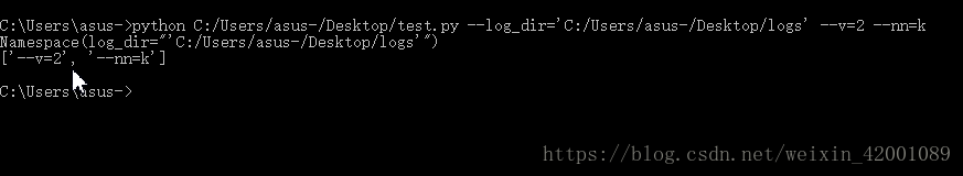
sys.argv[]就是一個從程式外部獲取引數的橋樑，sys.argv[0]就是返回第一個引數，即獲取當前指令碼

os.path.realpath就是獲取指令碼的絕對路徑

parser.parse_known_args()用 來解析不定長的命令列引數，其返回的是2個引數，第一個引數是已經定義了的引數，第二個是沒有定義的引數。

具體到這裡舉個例子就是：寫一個test.py

import argparse
import os
import sys

current_path = os.path.dirname(os.path.realpath(sys.argv[0]))

parser = argparse.ArgumentParser()
parser.add_argument(
    '--log_dir',
    type=str,
    default=os.path.join(current_path, 'log'),
    help='The log directory for TensorBoard summaries.')
FLAGS, unparsed = parser.parse_known_args()

print(FLAGS)
print(unparsed)

（三）接下來是下載資料集（這裡稍微做了一點修改）：

def maybe_download(filename, expected_bytes):
    """Download a file if not present, and make sure it's the right size."""
    if not os.path.exists(filename):
        filename, _ = urllib.request.urlretrieve(url + filename, filename)
    # 獲取檔案相關屬性
    statinfo = os.stat(filename)
    # 比對檔案的大小是否正確
    if statinfo.st_size == expected_bytes:
        print('Found and verified', filename)
    else:
        print(statinfo.st_size)
        raise Exception(
            'Failed to verify ' + filename + '. Can you get to it with a browser?')
    return filename

filename = maybe_download('text8.zip', 31344016)

下載好後就會在當前資料夾下有一個叫做text8.zip的壓縮包

（四）生成單詞表

# Read the data into a list of strings.
def read_data(filename):
  """Extract the first file enclosed in a zip file as a list of words."""
  with zipfile.ZipFile(filename) as f:
    data = tf.compat.as_str(f.read(f.namelist()[0])).split()
  return data


vocabulary = read_data(filename)
print('Data size', len(vocabulary))

f.namelist()[0]是解壓後第一個檔案，不過這裡解壓後本來就只有一個檔案，然後以空格分開，所以最後的vocabulary中就是單詞表，最後列印一下看看有多少單詞

(五)建立有50000個詞的字典，沒在該詞典的單詞用UNK表示 

vocabulary_size = 50000

def build_dataset(words, n_words):
  """Process raw inputs into a dataset."""
  count = [['UNK', -1]]
  count.extend(collections.Counter(words).most_common(n_words - 1))
  dictionary = dict()
  for word, _ in count:
    dictionary[word] = len(dictionary)
  data = list()
  unk_count = 0
  for word in words:
    index = dictionary.get(word, 0)
    if index == 0:  # dictionary['UNK']
      unk_count += 1
    data.append(index)
  count[0][1] = unk_count
  reversed_dictionary = dict(zip(dictionary.values(), dictionary.keys()))
  return data, count, dictionary, reversed_dictionary

data, count, dictionary, reverse_dictionary = build_dataset(
    vocabulary, vocabulary_size)
del vocabulary  # Hint to reduce memory.
print('Most common words (+UNK)', count[:5])
print('Sample data', data[:10], [reverse_dictionary[i] for i in data[:10]])

其中下面是統計每個單詞的詞頻，並選取前50000個詞頻較高的單詞作為字典的備選詞

extend追加一個列表

count.extend(collections.Counter(words).most_common(n_words - 1))

data是將資料集的單詞都編號，沒有在字典的中單詞編號為UNK(0)

就想這樣;

i    love   tensorflow  very  much .........

2    23      UNK           3       45    .........

count 記錄的是每個單詞對應的詞頻比如；[ ['UNK', -1] , ['a','200'] , ['i',150],...............]

dictionary是一個字典：記錄的是單詞對應編號 即key：單詞、value：編號(編號越小，詞頻越高，但第一個永遠是UNK)

reversed_dictionary是一個字典：編號對應的單詞  即key：編號、value：單詞(編號越小，詞頻越高，但第一個永遠是UNK)

第一個永遠是UNK是因為extend追加一個列表，變化的是追加的列表，第一個永遠是UNK

（六）取labels，分批次

data_index = 0

def generate_batch(batch_size, num_skips, skip_window):
  global data_index
  assert batch_size % num_skips == 0
  assert num_skips <= 2 * skip_window
  batch = np.ndarray(shape=(batch_size), dtype=np.int32)
  labels = np.ndarray(shape=(batch_size, 1), dtype=np.int32)
  span = 2 * skip_window + 1  # [ skip_window target skip_window ]
  buffer = collections.deque(maxlen=span)  # pylint: disable=redefined-builtin
  if data_index + span > len(data):
    data_index = 0
  buffer.extend(data[data_index:data_index + span])
  data_index += span
  for i in range(batch_size // num_skips):
    context_words = [w for w in range(span) if w != skip_window]
    words_to_use = random.sample(context_words, num_skips)
    for j, context_word in enumerate(words_to_use):
      batch[i * num_skips + j] = buffer[skip_window]
      labels[i * num_skips + j, 0] = buffer[context_word]
    if data_index == len(data):
      buffer.extend(data[0:span])
      data_index = span
    else:
      buffer.append(data[data_index])
      data_index += 1
  # Backtrack a little bit to avoid skipping words in the end of a batch
  data_index = (data_index + len(data) - span) % len(data)
  return batch, labels

batch, labels = generate_batch(batch_size=8, num_skips=2, skip_window=1)
for i in range(8):
  print(batch[i], reverse_dictionary[batch[i]], '->', labels[i, 0],
        reverse_dictionary[labels[i, 0]])

batch_size：就是批次大小

 num_skips：就是重複用一個單詞的次數，比如 num_skips=2時，對於一句話：i    love   tensorflow  very  much ..........

                        當tensorflow被選為目標詞時，在產生label時要利用tensorflow兩次即：

                         tensorflow---》 love        tensorflow---》 very

skip_window：是考慮左右上下文的個數，比如skip_window=1，就是在考慮上下文的時候，左面一個，右面一個

                           skip_window=2時，就是在考慮上下文的時候，左面兩個，右面兩個

 span ：其實在分批次的過程中可以看做是一個固定大小的框框（比較流行的說法數滑動視窗）在不斷移動，而這個框框的大小                  就是 span，可以看到span = 2 * skip_window + 1 

 buffer = collections.deque(maxlen=span)：就是申請了一個buffer（其實就是固定大小的視窗這裡是3）即每次這個buffer佇列中最                                                                           多 能容納span個單詞

所以過程應該是這樣的：比如batch_size=6， num_skips=2，skip_window=1，data:

batch_size // num_skips=3,迴圈3次

(   I      am      looking     for     the     missing     glass-shoes     who     has     picked   it      up .............)

    2      23        56            3       45         84               123              45        23           12     1     14 ...............

i=0時：2 ,23 ,56首先進入 buffer（ context_words = [w for w in range(span) if w != skip_window]的意思就是取視窗中不包括目標詞              的詞即上下文），然後batch[i * num_skips + j] = buffer[skip_window]（skip_window=1，所以每次就是取視窗的中間數為                目標詞）即batch=23，  labels[i * num_skips + j, 0] = buffer[context_word]就是取其上下文為labels即2和56

             所以此時batch=[23,23] labels=[2,56](當然也可能是[2,56]，因為可能先取右邊，後取左面)，同時data_index=3即單詞for的              位置

i=1時：data[data_index]進佇列，即 buffer為 23,56,3 賦值後為：batch=[23,23,56,56] labels=[2,56,23,3](也可能是換一下順序)

             同時data_index=4即單詞the

i=2時：data[data_index]進佇列，即 buffer為 56,3,45 賦值後為：batch=[23,23,56,56,3,3]  labels=[2,56,23,3,56,45](也可能是換一              下順序) 同時data_index=5即單詞missing

至此迴圈結束，按要求取出大小為6的一個批次即：

                                                batch=[23,23,56,56,3,3]                                labels=[2,56,23,3,56,45]

 然後data_index = (data_index + len(data) - span) % len(data)即data_index回溯3個單位，回到 looking,因為global data_index

所以data_index全域性變數，所以當在取下一個批次的時候，buffer從looking的位置開始裝載，即從上一個批次結束的位置接著往下取batch和labels

（七）定義一些引數大小：

batch_size = 128
embedding_size = 128  # Dimension of the embedding vector.
skip_window = 1  # How many words to consider left and right.
num_skips = 2  # How many times to reuse an input to generate a label.
num_sampled = 64  # Number of negative examples to sample.

graph = tf.Graph()

這裡主要就是定義我們上面講的一些引數的大小

（八）神經網路圖model：

with graph.as_default():

  # Input data.
  with tf.name_scope('inputs'):
    train_inputs = tf.placeholder(tf.int32, shape=[batch_size])
    train_labels = tf.placeholder(tf.int32, shape=[batch_size, 1])
    valid_dataset = tf.constant(valid_examples, dtype=tf.int32)

  # Ops and variables pinned to the CPU because of missing GPU implementation
  with tf.device('/cpu:0'):
    # Look up embeddings for inputs.
    with tf.name_scope('embeddings'):
      embeddings = tf.Variable(
          tf.random_uniform([vocabulary_size, embedding_size], -1.0, 1.0))
      embed = tf.nn.embedding_lookup(embeddings, train_inputs)

    # Construct the variables for the NCE loss
    with tf.name_scope('weights'):
      nce_weights = tf.Variable(
          tf.truncated_normal(
              [vocabulary_size, embedding_size],
              stddev=1.0 / math.sqrt(embedding_size)))
    with tf.name_scope('biases'):
      nce_biases = tf.Variable(tf.zeros([vocabulary_size]))

  # Compute the average NCE loss for the batch.
  # tf.nce_loss automatically draws a new sample of the negative labels each
  # time we evaluate the loss.
  # Explanation of the meaning of NCE loss:
  #   http://mccormickml.com/2016/04/19/word2vec-tutorial-the-skip-gram-model/
  with tf.name_scope('loss'):
    loss = tf.reduce_mean(
        tf.nn.nce_loss(
            weights=nce_weights,
            biases=nce_biases,
            labels=train_labels,
            inputs=embed,
            num_sampled=num_sampled,
            num_classes=vocabulary_size))

  # Add the loss value as a scalar to summary.
  tf.summary.scalar('loss', loss)

  # Construct the SGD optimizer using a learning rate of 1.0.
  with tf.name_scope('optimizer'):
    optimizer = tf.train.GradientDescentOptimizer(1.0).minimize(loss)

  # Compute the cosine similarity between minibatch examples and all embeddings.
  norm = tf.sqrt(tf.reduce_sum(tf.square(embeddings), 1, keepdims=True))
  normalized_embeddings = embeddings / norm
  valid_embeddings = tf.nn.embedding_lookup(normalized_embeddings,
                                            valid_dataset)
  similarity = tf.matmul(
      valid_embeddings, normalized_embeddings, transpose_b=True)

  # Merge all summaries.
  merged = tf.summary.merge_all()

  # Add variable initializer.
  init = tf.global_variables_initializer()

  # Create a saver.
  saver = tf.train.Saver()

這裡可以分為兩部分來看，一部分是訓練Skip-gram模型的詞向量，另一部分是計算餘弦相似度，下面我們分開說：

首先看下tf.nn.embedding_lookup的API解釋：

def embedding_lookup(
    params,
    ids,
    partition_strategy="mod",
    name=None,
    validate_indices=True,  # pylint: disable=unused-argument
    max_norm=None):
  """Looks up `ids` in a list of embedding tensors.
  This function is used to perform parallel lookups on the list of
  tensors in `params`.  It is a generalization of
  @{tf.gather}, where `params` is
  interpreted as a partitioning of a large embedding tensor.  `params` may be
  a `PartitionedVariable` as returned by using `tf.get_variable()` with a
  partitioner.
  If `len(params) > 1`, each element `id` of `ids` is partitioned between
  the elements of `params` according to the `partition_strategy`.
  In all strategies, if the id space does not evenly divide the number of
  partitions, each of the first `(max_id + 1) % len(params)` partitions will
  be assigned one more id.
  If `partition_strategy` is `"mod"`, we assign each id to partition
  `p = id % len(params)`. For instance,
  13 ids are split across 5 partitions as:
  `[[0, 5, 10], [1, 6, 11], [2, 7, 12], [3, 8], [4, 9]]`
  If `partition_strategy` is `"div"`, we assign ids to partitions in a
  contiguous manner. In this case, 13 ids are split across 5 partitions as:
  `[[0, 1, 2], [3, 4, 5], [6, 7, 8], [9, 10], [11, 12]]`
  The results of the lookup are concatenated into a dense
  tensor. The returned tensor has shape `shape(ids) + shape(params)[1:]`.

看到 The results of the lookup are concatenated into a dense tensor. The returned tensor has shape `shape(ids) + shape(params)[1:]`.，即假如params是:100*28,sp_ids是[2,56,3] 那麼返回的便是3*28即分別對應params的第3、57、4行

其實往下看會發現其主要呼叫的是 _embedding_lookup_and_transform函式

-----------------------------------------------------------------------------------------------------------------------------------------------------------------------------------

-----------------------------------------------------------------------------------------------------------------------------------------------------------------------------------

來重點看下tf.nn.nce_loss原始碼（這也是本demo中最核心的東西）：

def nce_loss(weights,
             biases,
             labels,
             inputs,
             num_sampled,
             num_classes,
             num_true=1,
             sampled_values=None,
             remove_accidental_hits=False,
             partition_strategy="mod",
             name="nce_loss"):
  """Computes and returns the noise-contrastive estimation training loss.
  See [Noise-contrastive estimation: A new estimation principle for
  unnormalized statistical
  models](http://www.jmlr.org/proceedings/papers/v9/gutmann10a/gutmann10a.pdf).
  Also see our [Candidate Sampling Algorithms
  Reference](https://www.tensorflow.org/extras/candidate_sampling.pdf)
  A common use case is to use this method for training, and calculate the full
  sigmoid loss for evaluation or inference. In this case, you must set
  `partition_strategy="div"` for the two losses to be consistent, as in the
  following example:
  ```python
  if mode == "train":
    loss = tf.nn.nce_loss(
        weights=weights,
        biases=biases,
        labels=labels,
        inputs=inputs,
        ...,
        partition_strategy="div")
  elif mode == "eval":
    logits = tf.matmul(inputs, tf.transpose(weights))
    logits = tf.nn.bias_add(logits, biases)
    labels_one_hot = tf.one_hot(labels, n_classes)
    loss = tf.nn.sigmoid_cross_entropy_with_logits(
        labels=labels_one_hot,
        logits=logits)
    loss = tf.reduce_sum(loss, axis=1)
  ```
  Note: By default this uses a log-uniform (Zipfian) distribution for sampling,
  so your labels must be sorted in order of decreasing frequency to achieve
  good results.  For more details, see
  @{tf.nn.log_uniform_candidate_sampler}.
  Note: In the case where `num_true` > 1, we assign to each target class
  the target probability 1 / `num_true` so that the target probabilities
  sum to 1 per-example.
  Note: It would be useful to allow a variable number of target classes per
  example.  We hope to provide this functionality in a future release.
  For now, if you have a variable number of target classes, you can pad them
  out to a constant number by either repeating them or by padding
  with an otherwise unused class.
  Args:
    weights: A `Tensor` of shape `[num_classes, dim]`, or a list of `Tensor`
        objects whose concatenation along dimension 0 has shape
        [num_classes, dim].  The (possibly-partitioned) class embeddings.
    biases: A `Tensor` of shape `[num_classes]`.  The class biases.
    labels: A `Tensor` of type `int64` and shape `[batch_size,
        num_true]`. The target classes.
    inputs: A `Tensor` of shape `[batch_size, dim]`.  The forward
        activations of the input network.
    num_sampled: An `int`.  The number of classes to randomly sample per batch.
    num_classes: An `int`. The number of possible classes.
    num_true: An `int`.  The number of target classes per training example.
    sampled_values: a tuple of (`sampled_candidates`, `true_expected_count`,
        `sampled_expected_count`) returned by a `*_candidate_sampler` function.
        (if None, we default to `log_uniform_candidate_sampler`)
    remove_accidental_hits:  A `bool`.  Whether to remove "accidental hits"
        where a sampled class equals one of the target classes.  If set to
        `True`, this is a "Sampled Logistic" loss instead of NCE, and we are
        learning to generate log-odds instead of log probabilities.  See
        our [Candidate Sampling Algorithms Reference]
        (https://www.tensorflow.org/extras/candidate_sampling.pdf).
        Default is False.
    partition_strategy: A string specifying the partitioning strategy, relevant
        if `len(weights) > 1`. Currently `"div"` and `"mod"` are supported.
        Default is `"mod"`. See `tf.nn.embedding_lookup` for more details.
    name: A name for the operation (optional).
  Returns:
    A `batch_size` 1-D tensor of per-example NCE losses.
  """
  logits, labels = _compute_sampled_logits(
      weights=weights,
      biases=biases,
      labels=labels,
      inputs=inputs,
      num_sampled=num_sampled,
      num_classes=num_classes,
      num_true=num_true,
      sampled_values=sampled_values,
      subtract_log_q=True,
      remove_accidental_hits=remove_accidental_hits,
      partition_strategy=partition_strategy,
      name=name)
  sampled_losses = sigmoid_cross_entropy_with_logits(
      labels=labels, logits=logits, name="sampled_losses")
  # sampled_losses is batch_size x {true_loss, sampled_losses...}
  # We sum out true and sampled losses.
  return _sum_rows(sampled_losses)

首先來看一下API:

def nce_loss(weights,
             biases,
             labels,
             inputs,
             num_sampled,
             num_classes,
             num_true=1,
             sampled_values=None,
             remove_accidental_hits=False,
             partition_strategy="mod",
             name="nce_loss"):

假如現在輸入資料是M*N（對應到我們這個demo就是說M=50000(詞典單詞數),N=128（word2vec的特徵數））

那麼：

weights：M*N

biases   :    N

labels    :   batch_size, num_true(num_true代表正樣本的數量，本demo中為1)

inputs    :   batch_size *N

num_sampled： 取樣的負樣本

num_classes ： M

sampled_values：是否用不同的取樣器，即tuple(`sampled_candidates`, `true_expected_count`  `sampled_expected_count`)

                              如果是None，這採用log_uniform_candidate_sampler

remove_accidental_hits:如果不下心採集到的負樣本就是target，要不要捨棄

partition_strategy:並行策略問題。

再看一下返回的就是

一個batch_size內每一個類子的NCE losses

下面看一下其實現，主要由三部分構成：

_compute_sampled_logits-----------------------取樣

sigmoid_cross_entropy_with_logits---------------------------logistic regression

_sum_rows------------------------------------------------------------求和。

（1）看一下_compute_sampled_logits

def _compute_sampled_logits(weights,
                            biases,
                            labels,
                            inputs,
                            num_sampled,
                            num_classes,
                            num_true=1,
                            sampled_values=None,
                            subtract_log_q=True,
                            remove_accidental_hits=False,
                            partition_strategy="mod",
                            name=None,
                            seed=None):
  """Helper function for nce_loss and sampled_softmax_loss functions.
  Computes sampled output training logits and labels suitable for implementing
  e.g. noise-contrastive estimation (see nce_loss) or sampled softmax (see
  sampled_softmax_loss).
  Note: In the case where num_true > 1, we assign to each target class
  the target probability 1 / num_true so that the target probabilities
  sum to 1 per-example.
  Args:
    weights: A `Tensor` of shape `[num_classes, dim]`, or a list of `Tensor`
        objects whose concatenation along dimension 0 has shape
        `[num_classes, dim]`.  The (possibly-partitioned) class embeddings.
    biases: A `Tensor` of shape `[num_classes]`.  The (possibly-partitioned)
        class biases.
    labels: A `Tensor` of type `int64` and shape `[batch_size,
        num_true]`. The target classes.  Note that this format differs from
        the `labels` argument of `nn.softmax_cross_entropy_with_logits_v2`.
    inputs: A `Tensor` of shape `[batch_size, dim]`.  The forward
        activations of the input network.
    num_sampled: An `int`.  The number of classes to randomly sample per batch.
    num_classes: An `int`. The number of possible classes.
    num_true: An `int`.  The number of target classes per training example.
    sampled_values: a tuple of (`sampled_candidates`, `true_expected_count`,
        `sampled_expected_count`) returned by a `*_candidate_sampler` function.
        (if None, we default to `log_uniform_candidate_sampler`)
    subtract_log_q: A `bool`.  whether to subtract the log expected count of
        the labels in the sample to get the logits of the true labels.
        Default is True.  Turn off for Negative Sampling.
    remove_accidental_hits:  A `bool`.  whether to remove "accidental hits"
        where a sampled class equals one of the target classes.  Default is
        False.
    partition_strategy: A string specifying the partitioning strategy, relevant
        if `len(weights) > 1`. Currently `"div"` and `"mod"` are supported.
        Default is `"mod"`. See `tf.nn.embedding_lookup` for more details.
    name: A name for the operation (optional).
    seed: random seed for candidate sampling. Default to None, which doesn't set
        the op-level random seed for candidate sampling.
  Returns:
    out_logits: `Tensor` object with shape
        `[batch_size, num_true + num_sampled]`, for passing to either
        `nn.sigmoid_cross_entropy_with_logits` (NCE) or
        `nn.softmax_cross_entropy_with_logits_v2` (sampled softmax).
    out_labels: A Tensor object with the same shape as `out_logits`.
  """

  if isinstance(weights, variables.PartitionedVariable):
    weights = list(weights)
  if not isinstance(weights, list):
    weights = [weights]

  with ops.name_scope(name, "compute_sampled_logits",
                      weights + [biases, inputs, labels]):
    if labels.dtype != dtypes.int64:
      labels = math_ops.cast(labels, dtypes.int64)
    labels_flat = array_ops.reshape(labels, [-1])

    # Sample the negative labels.
    #   sampled shape: [num_sampled] tensor
    #   true_expected_count shape = [batch_size, 1] tensor
    #   sampled_expected_count shape = [num_sampled] tensor
    if sampled_values is None:
      sampled_values = candidate_sampling_ops.log_uniform_candidate_sampler(
          true_classes=labels,
          num_true=num_true,
          num_sampled=num_sampled,
          unique=True,
          range_max=num_classes,
          seed=seed)
    # NOTE: pylint cannot tell that 'sampled_values' is a sequence
    # pylint: disable=unpacking-non-sequence
    sampled, true_expected_count, sampled_expected_count = (
        array_ops.stop_gradient(s) for s in sampled_values)
    # pylint: enable=unpacking-non-sequence
    sampled = math_ops.cast(sampled, dtypes.int64)

    # labels_flat is a [batch_size * num_true] tensor
    # sampled is a [num_sampled] int tensor
    all_ids = array_ops.concat([labels_flat, sampled], 0)

    # Retrieve the true weights and the logits of the sampled weights.

    # weights shape is [num_classes, dim]
    all_w = embedding_ops.embedding_lookup(
        weights, all_ids, partition_strategy=partition_strategy)

    # true_w shape is [batch_size * num_true, dim]
    true_w = array_ops.slice(all_w, [0, 0],
                             array_ops.stack(
                                 [array_ops.shape(labels_flat)[0], -1]))

    sampled_w = array_ops.slice(
        all_w, array_ops.stack([array_ops.shape(labels_flat)[0], 0]), [-1, -1])
    # inputs has shape [batch_size, dim]
    # sampled_w has shape [num_sampled, dim]
    # Apply X*W', which yields [batch_size, num_sampled]
    sampled_logits = math_ops.matmul(inputs, sampled_w, transpose_b=True)

    # Retrieve the true and sampled biases, compute the true logits, and
    # add the biases to the true and sampled logits.
    all_b = embedding_ops.embedding_lookup(
        biases, all_ids, partition_strategy=partition_strategy)
    # true_b is a [batch_size * num_true] tensor
    # sampled_b is a [num_sampled] float tensor
    true_b = array_ops.slice(all_b, [0], array_ops.shape(labels_flat))
    sampled_b = array_ops.slice(all_b, array_ops.shape(labels_flat), [-1])

    # inputs shape is [batch_size, dim]
    # true_w shape is [batch_size * num_true, dim]
    # row_wise_dots is [batch_size, num_true, dim]
    dim = array_ops.shape(true_w)[1:2]
    new_true_w_shape = array_ops.concat([[-1, num_true], dim], 0)
    row_wise_dots = math_ops.multiply(
        array_ops.expand_dims(inputs, 1),
        array_ops.reshape(true_w, new_true_w_shape))
    # We want the row-wise dot plus biases which yields a
    # [batch_size, num_true] tensor of true_logits.
    dots_as_matrix = array_ops.reshape(row_wise_dots,
                                       array_ops.concat([[-1], dim], 0))
    true_logits = array_ops.reshape(_sum_rows(dots_as_matrix), [-1, num_true])
    true_b = array_ops.reshape(true_b, [-1, num_true])
    true_logits += true_b
    sampled_logits += sampled_b

    if remove_accidental_hits:
      acc_hits = candidate_sampling_ops.compute_accidental_hits(
          labels, sampled, num_true=num_true)
      acc_indices, acc_ids, acc_weights = acc_hits

      # This is how SparseToDense expects the indices.
      acc_indices_2d = array_ops.reshape(acc_indices, [-1, 1])
      acc_ids_2d_int32 = array_ops.reshape(
          math_ops.cast(acc_ids, dtypes.int32), [-1, 1])
      sparse_indices = array_ops.concat([acc_indices_2d, acc_ids_2d_int32], 1,
                                        "sparse_indices")
      # Create sampled_logits_shape = [batch_size, num_sampled]
      sampled_logits_shape = array_ops.concat(
          [array_ops.shape(labels)[:1],
           array_ops.expand_dims(num_sampled, 0)], 0)
      if sampled_logits.dtype != acc_weights.dtype:
        acc_weights = math_ops.cast(acc_weights, sampled_logits.dtype)
      sampled_logits += sparse_ops.sparse_to_dense(
          sparse_indices,
          sampled_logits_shape,
          acc_weights,
          default_value=0.0,
          validate_indices=False)

    if subtract_log_q:
      # Subtract log of Q(l), prior probability that l appears in sampled.
      true_logits -= math_ops.log(true_expected_count)
      sampled_logits -= math_ops.log(sampled_expected_count)

    # Construct output logits and labels. The true labels/logits start at col 0.
    out_logits = array_ops.concat([true_logits, sampled_logits], 1)

    # true_logits is a float tensor, ones_like(true_logits) is a float
    # tensor of ones. We then divide by num_true to ensure the per-example
    # labels sum to 1.0, i.e. form a proper probability distribution.
    out_labels = array_ops.concat([
        array_ops.ones_like(true_logits) / num_true,
        array_ops.zeros_like(sampled_logits)
    ], 1)

    return out_logits, out_labels

首先看一下開頭註解的返回維數：

Returns:
    out_logits: `Tensor` object with shape
        `[batch_size, num_true + num_sampled]`, for passing to either
        `nn.sigmoid_cross_entropy_with_logits` (NCE) or
        `nn.softmax_cross_entropy_with_logits_v2` (sampled softmax).
    out_labels: A Tensor object with the same shape as `out_logits`.

即 返回的out_logits和 out_labels的維度都是[batch_size, num_true + num_sampled]，其中 num_true + num_sampled代表的就是正樣本數+負樣本數

再看一下最後：

out_labels = array_ops.concat([
        array_ops.ones_like(true_logits) / num_true,
        array_ops.zeros_like(sampled_logits)
    ], 1)

其中的array_ops.ones_like和array_ops.zeros_like就是賦值向量為全1和全0，也可以從下面的原始碼看到：

@tf_export("ones_like")
def ones_like(tensor, dtype=None, name=None, optimize=True):
  """Creates a tensor with all elements set to 1.
  Given a single tensor (`tensor`), this operation returns a tensor of the same
  type and shape as `tensor` with all elements set to 1. Optionally, you can
  specify a new type (`dtype`) for the returned tensor.
  For example:
  ```python
  tensor = tf.constant([[1, 2, 3], [4, 5, 6]])
  tf.ones_like(tensor)  # [[1, 1, 1], [1, 1, 1]]
  ```
  Args:
    tensor: A `Tensor`.
    dtype: A type for the returned `Tensor`. Must be `float32`, `float64`,
      `int8`, `uint8`, `int16`, `uint16`, `int32`, `int64`,
      `complex64`, `complex128` or `bool`.
    name: A name for the operation (optional).
    optimize: if true, attempt to statically determine the shape of 'tensor'
    and encode it as a constant.
  Returns:
    A `Tensor` with all elements set to 1.
  """
  with ops.name_scope(name, "ones_like", [tensor]) as name:
    tensor = ops.convert_to_tensor(tensor, name="tensor")
    ones_shape = shape_internal(tensor, optimize=optimize)
    if dtype is None:
      dtype = tensor.dtype
    ret = ones(ones_shape, dtype=dtype, name=name)
    if not context.executing_eagerly():
      ret.set_shape(tensor.get_shape())
    return ret

所以總結一下就是：

out_logits返回的就是目標詞彙

out_labels返回的就是正樣本+負樣本（其中正樣本都標記為1，負樣本都標記為0）

這也是負取樣的精髓所在，因為結果只有兩種結果，所以只做二分類就可以了，代替了之前需要預測整個詞典的大小，比如要對本類子中的50000種結果的每一種都預測，所以減少了計算的複雜度！！！！！！！！！！！！！！！

二者的維度都是[batch_size, num_true + num_sampled]

同時因為該demo中sampled_values=None，所以

if sampled_values is None:
      sampled_values = candidate_sampling_ops.log_uniform_candidate_sampler(
          true_classes=labels,
          num_true=num_true,
          num_sampled=num_sampled,
          unique=True,
          range_max=num_classes,
          seed=seed)

用到的是：candidate_sampling_ops.log_uniform_candidate_sampler取樣器

def log_uniform_candidate_sampler(true_classes, num_true, num_sampled, unique,
                                  range_max, seed=None, name=None):
  """Samples a set of classes using a log-uniform (Zipfian) base distribution.
  This operation randomly samples a tensor of sampled classes
  (`sampled_candidates`) from the range of integers `[0, range_max)`.
  The elements of `sampled_candidates` are drawn without replacement
  (if `unique=True`) or with replacement (if `unique=False`) from
  the base distribution.
  The base distribution for this operation is an approximately log-uniform
  or Zipfian distribution:
  `P(class) = (log(class + 2) - log(class + 1)) / log(range_max + 1)`
  This sampler is useful when the target classes approximately follow such
  a distribution - for example, if the classes represent words in a lexicon
  sorted in decreasing order of frequency. If your classes are not ordered by
  decreasing frequency, do not use this op.
  In addition, this operation returns tensors `true_expected_count`
  and `sampled_expected_count` representing the number of times each
  of the target classes (`true_classes`) and the sampled
  classes (`sampled_candidates`) is expected to occur in an average
  tensor of sampled classes.  These values correspond to `Q(y|x)`
  defined in [this
  document](http://www.tensorflow.org/extras/candidate_sampling.pdf).
  If `unique=True`, then these are post-rejection probabilities and we
  compute them approximately.
  Args:
    true_classes: A `Tensor` of type `int64` and shape `[batch_size,
      num_true]`. The target classes.
    num_true: An `int`.  The number of target classes per training example.
    num_sampled: An `int`.  The number of classes to randomly sample.
    unique: A `bool`. Determines whether all sampled classes in a batch are
      unique.
    range_max: An `int`. The number of possible classes.
    seed: An `int`. An operation-specific seed. Default is 0.
    name: A name for the operation (optional).
  Returns:
    sampled_candidates: A tensor of type `int64` and shape `[num_sampled]`.
      The sampled classes.
    true_expected_count: A tensor of type `float`.  Same shape as
      `true_classes`. The expected counts under the sampling distribution
      of each of `true_classes`.
    sampled_expected_count: A tensor of type `float`. Same shape as
      `sampled_candidates`. The expected counts under the sampling distribution
      of each of `sampled_candidates`.
  """
  seed1, seed2 = random_seed.get_seed(seed)
  return gen_candidate_sampling_ops.log_uniform_candidate_sampler(
      true_classes, num_true, num_sampled, unique, range_max, seed=seed1,
      seed2=seed2, name=name)

可以看到其對負樣本是基於以下概率取樣的，之所以不使用詞頻直接作為概率採用是因為如果這樣的話，那麼採取的負樣本就都會是哪些高頻詞彙類如：and , of , i 等等，顯然並不好。另一個極端就是使用詞頻的倒數，但是這對英文也沒有代表性，根據mikolov寫的一篇論文，實驗得出的經驗值是

這裡的話沒有用上面的公式，但是也使得其處於兩個極端之間了：還是可以看出P(class) 是遞減函式，即class越小，P(class)越大，class在本類中代表的是單詞的編號，由（五）可以知道，詞頻越大，編號越小（NUK除外），所以詞頻高的還是容易被作採用作為負樣本的！

P(class) = (log(class + 2) - log(class + 1)) / log(range_max + 1)

（2）接下來看一下sigmoid_cross_entropy_with_logits函式

def sigmoid_cross_entropy_with_logits(  # pylint: disable=invalid-name
    _sentinel=None,
    labels=None,
    logits=None,
    name=None):
  """Computes sigmoid cross entropy given `logits`.
  Measures the probability error in discrete classification tasks in which each
  class is independent and not mutually exclusive.  For instance, one could
  perform multilabel classification where a picture can contain both an elephant
  and a dog at the same time.
  For brevity, let `x = logits`, `z = labels`.  The logistic loss is
        z * -log(sigmoid(x)) + (1 - z) * -log(1 - sigmoid(x))
      = z * -log(1 / (1 + exp(-x))) + (1 - z) * -log(exp(-x) / (1 + exp(-x)))
      = z * log(1 + exp(-x)) + (1 - z) * (-log(exp(-x)) + log(1 + exp(-x)))
      = z * log(1 + exp(-x)) + (1 - z) * (x + log(1 + exp(-x))
      = (1 - z) * x + log(1 + exp(-x))
      = x - x * z + log(1 + exp(-x))
  For x < 0, to avoid overflow in exp(-x), we reformulate the above
        x - x * z + log(1 + exp(-x))
      = log(exp(x)) - x * z + log(1 + exp(-x))
      = - x * z + log(1 + exp(x))
  Hence, to ensure stability and avoid overflow, the implementation uses this
  equivalent formulation
      max(x, 0) - x * z + log(1 + exp(-abs(x)))
  `logits` and `labels` must have the same type and shape.
  Args:
    _sentinel: Used to prevent positional parameters. Internal, do not use.
    labels: A `Tensor` of the same type and shape as `logits`.
    logits: A `Tensor` of type `float32` or `float64`.
    name: A name for the operation (optional).
  Returns:
    A `Tensor` of the same shape as `logits` with the componentwise
    logistic losses.
  Raises:
    ValueError: If `logits` and `labels` do not have the same shape.
  """
  # pylint: disable=protected-access
  nn_ops._ensure_xent_args("sigmoid_cross_entropy_with_logits", _sentinel,
                           labels, logits)
  # pylint: enable=protected-access

  with ops.name_scope(name, "logistic_loss", [logits, labels]) as name:
    logits = ops.convert_to_tensor(logits, name="logits")
    labels = ops.convert_to_tensor(labels, name="labels")
    try:
      labels.get_shape().merge_with(logits.get_shape())
    except ValueError:
      raise ValueError("logits and labels must have the same shape (%s vs %s)" %
                       (logits.get_shape(), labels.get_shape()))

    # The logistic loss formula from above is
    #   x - x * z + log(1 + exp(-x))
    # For x < 0, a more numerically stable formula is
    #   -x * z + log(1 + exp(x))
    # Note that these two expressions can be combined into the following:
    #   max(x, 0) - x * z + log(1 + exp(-abs(x)))
    # To allow computing gradients at zero, we define custom versions of max and
    # abs functions.
    zeros = array_ops.zeros_like(logits, dtype=logits.dtype)
    cond = (logits >= zeros)
    relu_logits = array_ops.where(cond, logits, zeros)
    neg_abs_logits = array_ops.where(cond, -logits, logits)
    return math_ops.add(
        relu_logits - logits * labels,
        math_ops.log1p(math_ops.exp(neg_abs_logits)),
        name=name)

可以看到其實最關鍵的就是下面這個公式：

z * -log(sigmoid(x)) + (1 - z) * -log(1 - sigmoid(x))

其實z * -log(x) + (1 - z) * -log(1 - x)就是交叉熵，對的，沒看錯這個函式其實就是將輸入先sigmoid再計算交叉熵

如上所示最後化簡結果為：x - x * z + log(1 + exp(-x))

這裡考慮到當x<0時exp(-x)有可能溢位，所以當x<0時有- x * z + log(1 + exp(x))

最後綜合兩種情況歸納出：

 max(x, 0) - x * z + log(1 + exp(-abs(x)))

關於交叉熵的概念可以看一下：

（3）最後看一下_sum_rows

def _sum_rows(x):
  """Returns a vector summing up each row of the matrix x."""
  # _sum_rows(x) is equivalent to math_ops.reduce_sum(x, 1) when x is
  # a matrix.  The gradient of _sum_rows(x) is more efficient than
  # reduce_sum(x, 1)'s gradient in today's implementation. Therefore,
  # we use _sum_rows(x) in the nce_loss() computation since the loss
  # is mostly used for training.
  cols = array_ops.shape(x)[1]
  ones_shape = array_ops.stack([cols, 1])
  ones = array_ops.ones(ones_shape, x.dtype)
  return array_ops.reshape(math_ops.matmul(x, ones), [-1])

這個相當簡單了就是將矩陣的每一行都加起來，即根據上面的[batch_size, num_true + num_sampled]，其實就是true loss與 sampled loss之和，即求batch_size中每一個example的總loss

到此tf.nn.nce_loss就結束了，這就是最重要的部分

-----------------------------------------------------------------------------------------------------------------------------------------------------------------------------

-----------------------------------------------------------------------------------------------------------------------------------------------------------------------------------

從程式碼可以看出這裡選擇的 optimizer是GradientDescentOptimizer，然後就是通過normalized_embeddings = embeddings / norm

對word2vec矩陣進行了歸一化

下面接著上面來看一下計算餘弦相似度的部分

valid_embeddings = tf.nn.embedding_lookup(normalized_embeddings,
                                            valid_dataset)
  similarity = tf.matmul(
      valid_embeddings, normalized_embeddings, transpose_b=True)

這裡很簡單，這裡就是抽取其中valid_dataset個詞向量計算餘弦相似度，餘弦相似度就是通過兩個向量的夾角的餘弦值來衡量相似程度，顯然當角度為0時，二者重合，最相近，此時其餘弦值也最大為1，本demo中抽取的方式是從前100個詞頻最高的詞中選取隨機選取16個即：

valid_size = 16  # Random set of words to evaluate similarity on.
valid_window = 100  # Only pick dev samples in the head of the distribution.
valid_examples = np.random.choice(valid_window, valid_size, replace=False)

（九）建立會話

num_steps = 100001

with tf.Session(graph=graph) as session:
  # Open a writer to write summaries.
  writer = tf.summary.FileWriter(FLAGS.log_dir, session.graph)

  # We must initialize all variables before we use them.
  init.run()
  print('Initialized')

  average_loss = 0
  for step in xrange(num_steps):
    batch_inputs, batch_labels = generate_batch(batch_size, num_skips,
                                                skip_window)
    feed_dict = {train_inputs: batch_inputs, train_labels: batch_labels}

    # Define metadata variable.
    run_metadata = tf.RunMetadata()

    # We perform one update step by evaluating the optimizer op (including it
    # in the list of returned values for session.run()
    # Also, evaluate the merged op to get all summaries from the returned "summary" variable.
    # Feed metadata variable to session for visualizing the graph in TensorBoard.
    _, summary, loss_val = session.run(
        [optimizer, merged, loss],
        feed_dict=feed_dict,
        run_metadata=run_metadata)
    average_loss += loss_val

    # Add returned summaries to writer in each step.
    writer.add_summary(summary, step)
    # Add metadata to visualize the graph for the last run.
    if step == (num_steps - 1):
      writer.add_run_metadata(run_metadata, 'step%d' % step)

    if step % 2000 == 0:
      if step > 0:
        average_loss /= 2000
      # The average loss is an estimate of the loss over the last 2000 batches.
      print('Average loss at step ', step, ': ', average_loss)
      average_loss = 0

    # Note that this is expensive (~20% slowdown if computed every 500 steps)
    if step % 10000 == 0:
      sim = similarity.eval()
      for i in xrange(valid_size):
        valid_word = reverse_dictionary[valid_examples[i]]
        top_k = 8  # number of nearest neighbors
        nearest = (-sim[i, :]).argsort()[1:top_k + 1]
        log_str = 'Nearest to %s:' % valid_word
        for k in xrange(top_k):
          close_word = reverse_dictionary[nearest[k]]
          log_str = '%s %s,' % (log_str, close_word)
        print(log_str)
  final_embeddings = normalized_embeddings.eval()

  # Write corresponding labels for the embeddings.
  with open(FLAGS.log_dir + '/metadata.tsv', 'w') as f:
    for i in xrange(vocabulary_size):
      f.write(reverse_dictionary[i] + '\n')

  # Save the model for checkpoints.
  saver.save(session, os.path.join(FLAGS.log_dir, 'model.ckpt'))

  # Create a configuration for visualizing embeddings with the labels in TensorBoard.
  config = projector.ProjectorConfig()
  embedding_conf = config.embeddings.add()
  embedding_conf.tensor_name = embeddings.name
  embedding_conf.metadata_path = os.path.join(FLAGS.log_dir, 'metadata.tsv')
  projector.visualize_embeddings(writer, config)

writer.close()

這部分原始碼簡單易懂主要依次做了以下幾件事：

（1）訓練模型

（2）在訓練最後一次，儲存模型用以後續視覺化

（3）每2000次，計算一次平均loss

（4）每10000次，列印（八）中隨機選取16個詞各自對應的與其最相近的8個詞

（5）儲存訓練好的embeddings矩陣為.tsv格式用於在tensorboard通過降維來視覺化

（6）儲存模型為.ckpt

（十）二維視覺化

def plot_with_labels(low_dim_embs, labels, filename):
  assert low_dim_embs.shape[0] >= len(labels), 'More labels than embeddings'
  plt.figure(figsize=(18, 18))  # in inches
  for i, label in enumerate(labels):
    x, y = low_dim_embs[i, :]
    plt.scatter(x, y)
    plt.annotate(
        label,
        xy=(x, y),
        xytext=(5, 2),
        textcoords='offset points',
        ha='right',
        va='bottom')

  plt.savefig(filename)


try:
  # pylint: disable=g-import-not-at-top
  from sklearn.manifold import TSNE
  import matplotlib.pyplot as plt

  tsne = TSNE(
      perplexity=30, n_components=2, init='pca', n_iter=5000, method='exact')
  plot_only = 500
  low_dim_embs = tsne.fit_transform(final_embeddings[:plot_only, :])
  labels = [reverse_dictionary[i] for i in xrange(plot_only)]
  plot_with_labels(low_dim_embs, labels, os.path.join(FLAGS.log_dir, 'tsne.png', 'tsne.png'))

except ImportError as ex:
  print('Please install sklearn, matplotlib, and scipy to show embeddings.')
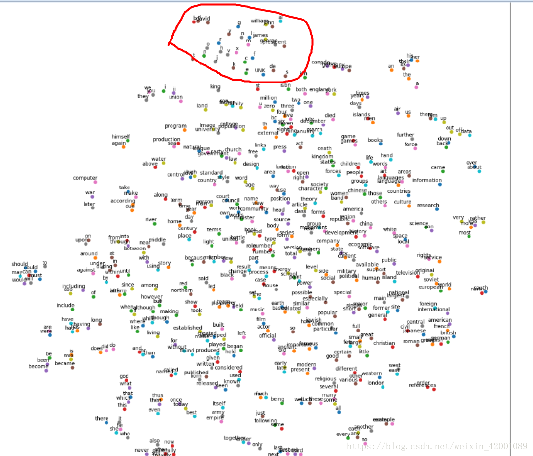
  print(ex)

這裡其實歸結起來就是做了一件事那就是：將訓練好的embeddings降為2維，然後儲存為圖片形式用於視覺化

這裡只選擇了embeddings前500個用於視覺化，重點就是使用TSNE這個包用於降為

這裡簡單說一下引數：

 perplexity為浮點型，可選（預設：30）較大的資料集通常需要更大的perplexity

n_components 降為幾維，預設2

init 可選嵌入的初始化，預設值：“random”，這裡選取pca是因為其通常比隨機初始化更全域性穩定。但需要注意的是pca初始化不         能用於預先計算的距離

n_iter 優化的最大迭代次數

method  梯度計算演算法使用在O（NlogN）時間內執行的Barnes-Hut近似值。 method ='exact'將執行在O（N ^ 2）時間內較慢但精確的演算法上。當最近鄰的誤差需要好於3％時，應該使用精確的演算法。但是，確切的方法無法擴充套件到數百萬個示例。0.17新版​​功能：通過Barnes-Hut近似優化方法。

更多引數可以參考：

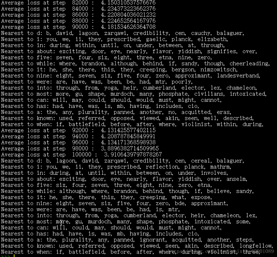
到這裡原始碼講解完畢，下面是執行結果的部分截圖：

可以看到詞頻最高的幾個詞以及其詞頻分別為：

Most common words (+UNK) [['UNK', 418391], ('the', 1061396), ('of', 593677), ('and', 416629), ('one', 411764)]

然後是去了文章十個單詞以及其對應的編號：

Sample data [5234, 3081, 12, 6, 195, 2, 3134, 46, 59, 156] ['anarchism', 'originated', 'as', 'a', 'term', 'of', 'abuse', 'first', 'used', 'against']

然後是取了一個批次，其大小為8，列印了其目標詞彙以及上下文：

3081 originated -> 5234 anarchism
3081 originated -> 12 as
12 as -> 6 a
12 as -> 3081 originated
6 a -> 195 term
6 a -> 12 as
195 term -> 2 of
195 term -> 6 a

從這裡也可以看到每個目標詞彙被用了2次

接下來就是一次次的迭代，我們看最後一次的：

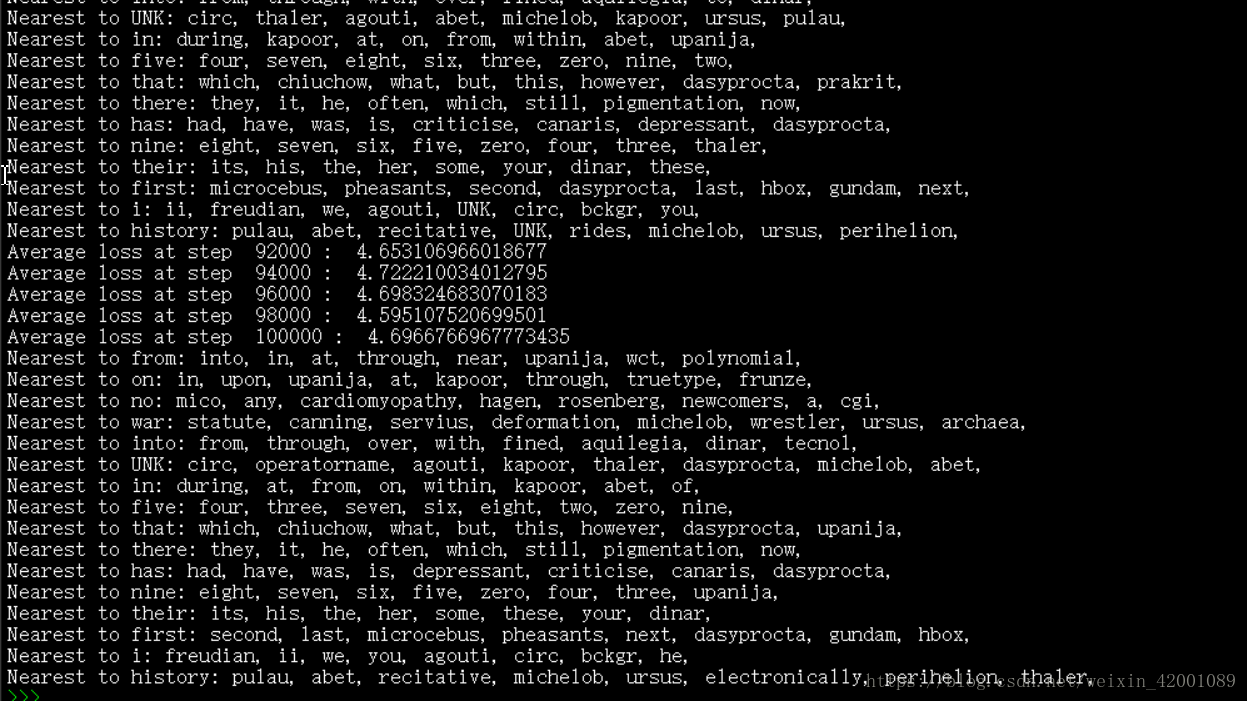
可以看到最和from接近的詞彙有into, in, at, through, near, upanija, wct, polynomial

和five接近的詞彙有 four, three, seven, six, eight, two, zero, nine等等

總之結果還是比較好的

看一下上圖視覺化的二維的圖片，比如紅圈都是助動詞

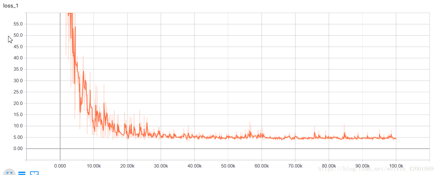
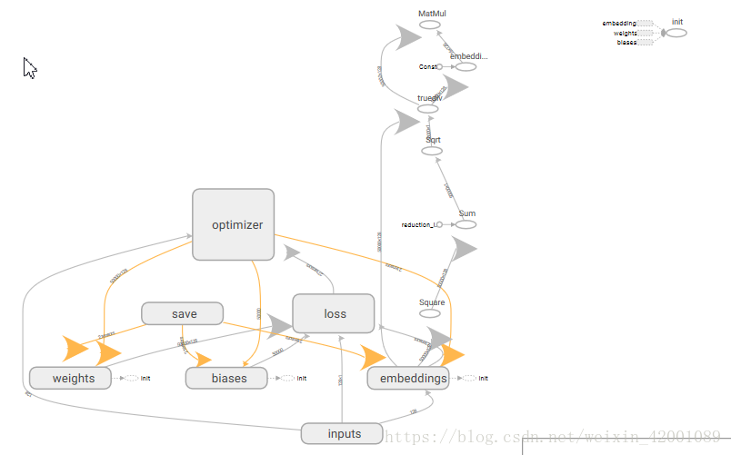
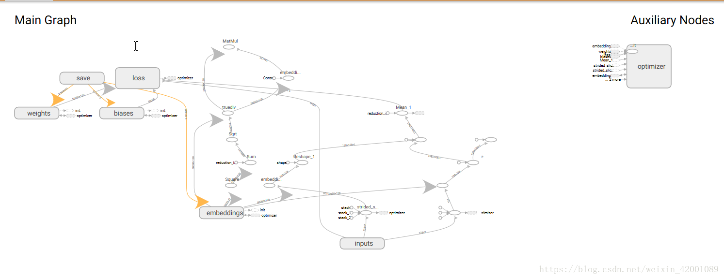
再來看一下tensorboard中的視覺化

###################################################################################################

以上就是word2vec的Skip-Gram模型，下面介紹CBOW

對比以上Skip-Gram模型：

當CBOW_window=1時：

I      am      looking     for     the     missing     glass-shoes     who     has     picked   it      up .............

batch：[ ' i ' , ' looking '] , [ ' am ' , ' for '] , [ ' looking ' , ' the '] , [ ' for ' , ' missing '] .................

labels: [ ' am '  ,  ' looking ' ,  ' for '  ,  ' the ' ] 

所以首先要改的就是將上面的(六)（八）部分改為：

def generate_batch(batch_size, cbow_window):
    global data_index
    assert cbow_window % 2 == 1
    span = 2 * cbow_window + 1
    # 去除中心word: span - 1
    batch = np.ndarray(shape=(batch_size, span - 1), dtype=np.int32)
    labels = np.ndarray(shape=(batch_size, 1), dtype=np.int32)

    buffer = collections.deque(maxlen=span)
    for _ in range(span):
        buffer.append(data[data_index])
        # 迴圈選取 data中資料，到尾部則從頭開始
        data_index = (data_index + 1) % len(data)
    
    for i in range(batch_size):
        # target at the center of span
        target = cbow_window
        # 僅僅需要知道context(word)而不需要word
        target_to_avoid = [cbow_window]

        col_idx = 0
        for j in range(span):
            # 略過中心元素 word
            if j == span // 2:
                continue
            batch[i, col_idx] = buffer[j]
            col_idx += 1
        labels[i, 0] = buffer[target]
        # 更新 buffer
        buffer.append(data[data_index])
        data_index = (data_index + 1) % len(data)

    return batch, labels



batch, labels = generate_batch(batch_size=8, cbow_window=1)
for i in range(8):
  print(reverse_dictionary[batch[i,0]],'and',reverse_dictionary[batch[i,1]] ,'->', 
        reverse_dictionary[labels[i, 0]])

with graph.as_default():

  # Input data.
  with tf.name_scope('inputs'):

    train_dataset = tf.placeholder(tf.int32, shape=[batch_size,2 * cbow_window])
    train_labels = tf.placeholder(tf.int32, shape=[batch_size, 1])
    valid_dataset = tf.constant(valid_examples, dtype=tf.int32)



  # Ops and variables pinned to the CPU because of missing GPU implementation
  with tf.device('/cpu:0'):
    # Look up embeddings for inputs.
    with tf.name_scope('embeddings'):
      embeddings = tf.Variable(
          tf.random_uniform([vocabulary_size, embedding_size], -1.0, 1.0))


    # Construct the variables for the NCE loss
    with tf.name_scope('weights'):
      nce_weights = tf.Variable(
          tf.truncated_normal(
              [vocabulary_size, embedding_size],
              stddev=1.0 / math.sqrt(embedding_size)))
    with tf.name_scope('biases'):
      nce_biases = tf.Variable(tf.zeros([vocabulary_size]))



  embeds = None
  for i in range(2 * cbow_window):
    embedding_i = tf.nn.embedding_lookup(embeddings, train_dataset[:,i])
    print('embedding %d shape: %s'%(i, embedding_i.get_shape().as_list()))
    emb_x,emb_y = embedding_i.get_shape().as_list()
    if embeds is None:
      
      embeds = tf.reshape(embedding_i, [emb_x,emb_y,1])
    else:
      embeds = tf.concat([embeds, tf.reshape(embedding_i, [emb_x, emb_y,1])], 2)
    print("Concat embedding size: %s"%embeds.get_shape().as_list())
    avg_embed =  tf.reduce_mean(embeds, 2, keep_dims=False)
    print("Avg embedding size: %s"%avg_embed.get_shape().as_list())
  print('--------------------------------------------------------------------------------------------')
  print(avg_embed.shape)
  print(train_labels.shape)
  print('--------------------------------------------------------------------------------------------')
  # Compute the average NCE loss for the batch.
  # tf.nce_loss automatically draws a new sample of the negative labels each
  # time we evaluate the loss.
  # Explanation of the meaning of NCE loss:
  #   http://mccormickml.com/2016/04/19/word2vec-tutorial-the-skip-gram-model/
  with tf.name_scope('loss'):
    loss = tf.reduce_mean(
        tf.nn.nce_loss(
            weights=nce_weights,
            biases=nce_biases,
            labels=train_labels,
            inputs=avg_embed,
            num_sampled=num_sampled,
            num_classes=vocabulary_size))

  # Add the loss value as a scalar to summary.
  tf.summary.scalar('loss', loss)

  # Construct the SGD optimizer using a learning rate of 1.0.
  with tf.name_scope('optimizer'):
    optimizer = tf.train.GradientDescentOptimizer(1.0).minimize(loss)

  # Compute the cosine similarity between minibatch examples and all embeddings.
  norm = tf.sqrt(tf.reduce_sum(tf.square(embeddings), 1, keepdims=True))
  normalized_embeddings = embeddings / norm
  valid_embeddings = tf.nn.embedding_lookup(normalized_embeddings,
                                            valid_dataset)
  similarity = tf.matmul(
      valid_embeddings, normalized_embeddings, transpose_b=True)

  # Merge all summaries.
  merged = tf.summary.merge_all()

  # Add variable initializer.
  init = tf.global_variables_initializer()

  # Create a saver.
  saver = tf.train.Saver()

這裡的特殊之處在於怎麼將batch和labels維數對應

以下假設embeding的特徵數都是128

對於Skip-Gram模型模型

經過generate_batch後返回：

batch：batch_size

labels : batch_size*1

然後 經過（八）的（train_inputs=batch） embed = tf.nn.embedding_lookup(embeddings, train_inputs)後

embed : batch_size*128

labels : batch_size*1

所以傳給 tf.nn.nce_loss進行訓練的

此時對於CBOW模型

經過generate_batch後返回：

batch：batch_size*span - 1（batch_size*2）

labels : batch_size*1

如果還是按照Skip-Gram模型則

 經過（八）的（train_inputs=batch） embed = tf.nn.embedding_lookup(embeddings, train_inputs)後

會報錯，而且原先Skip-Gram中目標詞彙是一個，現在CBOW中目標詞彙是兩個

基於此本程式是進行如下處理來產生embed 的：

首先先遍歷目標詞彙的一個（i=0），通過 embedding_i = tf.nn.embedding_lookup(embeddings, train_dataset[:,i])

此時embedding_i維度為batch_size*128然後reshape為batch_size*128*1

然後將embedding_i賦給 embeds

接著再遍歷目標詞中剩下的一個（i=1）,通過 embedding_i = tf.nn.embedding_lookup(embeddings, train_dataset[:,i])

此時embedding_i維度為batch_size*128然後reshape為batch_size*128*1

然後再將embedding_i合併到embeds（合併的維度是2）此時embeds維度為batch_size*128*2

然後avg_embed =  tf.reduce_mean(embeds, 2, keep_dims=False)後avg_embed維數為batch_size*128

最後將

avg_embed : batch_size*128

labels： batch_size*1

所以傳給 tf.nn.nce_loss進行訓練的

這樣說不是很直觀下面舉個類子（batch_size=8）

即比如batch為[ [ 1 , 2 ] , [ 3 , 4 ], [ 5 , 6 ], [ 7 , 8 ], [ 9 , 10 ], [ 11 , 12 ], [ 13 , 14 ], [ 15 , 16 ]]

embeddings為 [  [ 1.1 , 1.2  ,1.3 ,.....................................................1.128]

                              [ 2.1 , 2.2  ,2.3 ,.....................................................2.128]

                              [ 3.1 , 3.2  ,3.3 ,.....................................................3.128]

                              ................................

                              [ 50000.1 , 50000.2  ,50000.3 ,..................50000.128]

                             ]

那麼embeds為   [   [  [1.1 , 2.1] , [1.2 , 2.2] , [1.3 , 2.3] .......... , [1.128 , 2.128]  ]  

                                 [  [3.1 , 4.1] , [3.2 , 4.2] , [3.3 , 4.3] .......... , [3.128 , 4.128]  ]  

                                 [  [5.1 , 6.1] , [5.2 ,6.2] , [5.3 , 6.3] .......... , [5.128 , 6.128]  ]  

                                 [  [7.1 , 8.1] , [7.2 , 8.2] , [7.3 , 8.3] .......... , [7.128 , 8.128]  ]  

                                 [  [9.1 , 10.1] , [9.2 , 10.2] , [9.3 , 10.3] .......... , [9.128 , 10.128]  ]  

                                 [  [11.1 , 12.1] , [11.2 , 12.2] , [11.3 , 12.3] .......... , [11.128 , 12.128]  ]  

                                 [  [13.1 , 14.1] , [13.2 , 14.2] , [13.3 , 14.3] .......... , [13.128 , 14.128]  ]  

                                 [  [15.1 , 16.1] , [15.2 , 16.2] , [15.3 , 16.3] .......... , [15.128 , 16.128]  ]  

                                ]

avg_embed為  

                             [   [  [ 3.2 ] , [ 3.4 ] , [ 3.6 ]  .......... , [ 3.256 ]  ]  

                                 [  [ 7.2 ] , [ 7.4 ] , [ 7.6 ] .......... , [ 7.256 ]  ]  

                                 [  [ 11.2 ] , [ 11.4 ] , [11.6 ] .......... , [ 11.256 ]  ]  

                                 .........................

                                 [  [ 31.2 ] , [ 31.4 ] , [ 31.6 ] .......... , [ 31.256 ]  ]  

                                ]

可以看出CBOW模型其實就是將目標詞彙中的兩個詞對應的128個特徵分別相加，整體作為一個輸入的

其他程式碼就與Skip-Gram模型基本相同了

-----------------------------------------------------------------------------------------------------------------------------------------------------------------------------------

以下為執行結果的部分截圖：

可以看到最後一步的loss為3.91,而Skip-Gram最後一步的loss為4.69，所以CBOW模型訓練的結果更好一點，是因為其同時考慮了兩個詞去預測一個詞，而Skip-Gram是用一個詞去預測上下文

視覺化也可以看到結果

tensorboard中的視覺化：

相關推薦