學習記錄：一個試卷批改系統

阿新 • • 發佈：2019-01-22

本文程式設計採用Python語言，結合opencv庫對影象進行處理，再利用TensorFlow框架下卷積神經網路實現一個初步的簡易試卷批改系統。
實現一個試卷批改系統，我將它主要分成倆個模組，第一個模組是影象識別，第二個模組是利用機器學習訓練模型。
先說我們是如何訓練模型的，對於一般的影象分類問題，利用卷積神經網路是一個不錯的選擇，卷積神經網路在影象分類的應用十分廣泛，具體程式碼如下：

import tensorflow as tf
from tensorflow.examples.tutorials.mnist import input_data
mnist=input_data.read_data_sets('MNIST_data' 
,one_hot=True)#下載mnist資料集
def compute_accuracy(v_xs,v_ys):
    global prediction#定義全域性變數
    y_pre=sess.run(prediction,feed_dict={xs:v_xs,keep_prob:1})#
    correct_prediction=tf.equal(tf.argmax(y_pre,1),tf.argmax(v_ys,1))#將實際值和預測值進行比較，返回Bool資料型別
    accuracy=tf.reduce_mean(tf.cast(correct_prediction,tf.float32))#將上面的bool型別轉為float，求得矩陣中所有元素的平均值 

    result=sess.run(accuracy,feed_dict={xs:v_xs,ys:v_ys,keep_prob:1})#執行得到上面的平均值，這個值越大說明預測的越準確，因為都是0-1型別，所以平均值不超過1
    return result
def weight_variable(shape):
    initial=tf.truncated_normal(shape,stddev=0.1)#這個函式產生的隨機數與均值的差距不會超過兩倍的標準差
    return tf.Variable(initial,dtype=tf.float32,name='weight')
def 
 bias_variable(shape):
    initial=tf.constant(0.1,shape=shape)
    return tf.Variable(initial,dtype=tf.float32,name='biases')
def conv2d(x,W):
    return tf.nn.conv2d(x,W,strides=[1,1,1,1],padding='SAME')#strides第一個和第四個都是1，然後中間倆個代表x方向和y方向的步長,這個函式用來定義卷積神經網路
def max_pool_2x2(x):
    return tf.nn.max_pool(x,ksize=[1,2,2,1],strides=[1,2,2,1],padding='SAME')


xs=tf.placeholder(tf.float32,[None,784])#輸入是一個28*28的畫素點的資料
ys=tf.placeholder(tf.float32,[None,10])
keep_prob=tf.placeholder(tf.float32)

x_image=tf.reshape(xs,[-1,28,28,1])#xs的維度暫時不管，用-1表示，28,28表示xs的資料，1表示該資料是一個黑白照片，如果是彩色的，則寫成3
#卷積層1
W_conv1=weight_variable([5,5,1,32])#抽取一個5*5畫素，高度是32的點,每次抽出原影象的5*5的畫素點，高度從1變成32
b_conv1=bias_variable([32])
h_conv1=tf.nn.relu(conv2d(x_image,W_conv1)+b_conv1)#輸出 28*28*32的影象
h_pool1=max_pool_2x2(h_conv1)##輸出14*14*32的影象，因為這個函式的步長是2*2，影象縮小一半。
#卷積層2
W_conv2=weight_variable([5,5,32,64])#隨機生成一個5*5畫素，高度是64的點,抽出原影象的5*5的畫素點，高度從32變成64
b_conv2=bias_variable([64])
h_conv2=tf.nn.relu(conv2d(h_pool1,W_conv2)+b_conv2)#輸出14*14*64的影象
h_pool2=max_pool_2x2(h_conv2)##輸出7*7*64的影象，因為這個函式的步長是2*2，影象縮小一半。
#fully connected 1
W_fc1=weight_variable([7*7*64,1024])
b_fc1=bias_variable([1024])
h_pool2_flat=tf.reshape(h_pool2,[-1,7*7*64])#將輸出的h_pool2的三維資料變成一維資料，平鋪下來，（-1）代表的是有多少個例子
h_fc1=tf.nn.relu(tf.matmul(h_pool2_flat,W_fc1)+b_fc1)
h_fc1_drop=tf.nn.dropout(h_fc1,keep_prob)
#fully connected 2
W_fc2=weight_variable([1024,10])
b_fc2=bias_variable([10])
prediction=tf.nn.softmax(tf.matmul(h_fc1_drop,W_fc2)+b_fc2)#輸出層

#開始訓練資料
cross_entropy=tf.reduce_mean(-tf.reduce_sum(ys*tf.log(prediction),reduction_indices=[1]))#相當於loss（代價函式）
train_step=tf.train.AdamOptimizer(1e-4).minimize(cross_entropy)#訓練函式，降低cross_entropy（loss）,AdamOptimizer適用於大的神經網路
saver = tf.train.Saver()
with tf.Session() as sess:
    sess.run(tf.global_variables_initializer())

    for i in range(10000):
        batch_xs,batch_ys=mnist.train.next_batch(250)#每次從mnist資料集裡面拿100個數據訓練
        sess.run(train_step,feed_dict={xs:batch_xs,ys:batch_ys,keep_prob:0.5})
        if i%100==0:
            print(compute_accuracy(mnist.test.images,mnist.test.labels))
    save_path = saver.save(sess, "my_net/save_net.ckpt)

測試下我們訓練的準確率情況:訓練10000次，每隔100次列印一次，最後的訓練準確率大概是99%左右。

程式碼中使用的是mnist手寫數字資料集，將影象分成10個類別，分別代表數字0-9，訓練好的模型儲存在my_net/save_net.ckpt裡面，檔案格式是.ckpt。
下一步工作是如何呼叫訓練的模型。呼叫模型的方法很簡單，首先需要重構一個和訓練集一樣的神經網路架構，注意這裡不需要再訓練資料了，直接呼叫模型就可以了，然後輸入和mnist資料集相同格式的圖片就能實現數字識別。如下程式碼是如何重構模型以及呼叫模型的方法。（注意在儲存和呼叫模型的程式碼中均有saver.restore(sess, “my_net/save_net.ckpt”)這段程式碼，唯一不同的是，儲存程式碼用的是saver.save(sess, “my_net/save_net.ckpt”)，呼叫程式碼用的是saver.restore(sess, “my_net/save_net.ckpt”)。）

import tensorflow as tf
import cv2
from PIL import Image
import numpy as np
def weight_variable(shape):
    initial=tf.truncated_normal(shape,stddev=0.1)
    return tf.Variable(initial,dtype=tf.float32,name='weight')
def bias_variable(shape):
    initial=tf.constant(0.1,shape=shape)
    return tf.Variable(initial,dtype=tf.float32,name='biases')
def conv2d(x,W):
    return tf.nn.conv2d(x,W,strides=[1,1,1,1],padding='SAME')
def max_pool_2x2(x):
    return tf.nn.max_pool(x,ksize=[1,2,2,1],strides=[1,2,2,1],padding='SAME')

xs=tf.placeholder(tf.float32,[None,784])#輸入是一個28*28的畫素點的資料

keep_prob=tf.placeholder(tf.float32)

x_image=tf.reshape(xs,[-1,28,28,1])#xs的維度暫時不管，用-1表示，28,28表示xs的資料，1表示該資料是一個黑白照片，如果是彩色的，則寫成3
#卷積層1
W_conv1=weight_variable([5,5,1,32])#抽取一個5*5畫素，高度是32的點,每次抽出原影象的5*5的畫素點，高度從1變成32
b_conv1=bias_variable([32])
h_conv1=tf.nn.relu(conv2d(x_image,W_conv1)+b_conv1)#輸出 28*28*32的影象
h_pool1=max_pool_2x2(h_conv1)##輸出14*14*32的影象，因為這個函式的步長是2*2，影象縮小一半。
#卷積層2
W_conv2=weight_variable([5,5,32,64])#隨機生成一個5*5畫素，高度是64的點,抽出原影象的5*5的畫素點，高度從32變成64
b_conv2=bias_variable([64])
h_conv2=tf.nn.relu(conv2d(h_pool1,W_conv2)+b_conv2)#輸出14*14*64的影象
h_pool2=max_pool_2x2(h_conv2)##輸出7*7*64的影象，因為這個函式的步長是2*2，影象縮小一半。
#fully connected 1
W_fc1=weight_variable([7*7*64,1024])
b_fc1=bias_variable([1024])
h_pool2_flat=tf.reshape(h_pool2,[-1,7*7*64])#將輸出的h_pool2的三維資料變成一維資料，平鋪下來，（-1）代表的是有多少個例子
h_fc1=tf.nn.relu(tf.matmul(h_pool2_flat,W_fc1)+b_fc1)
h_fc1_drop=tf.nn.dropout(h_fc1,keep_prob)
#fully connected 2
W_fc2=weight_variable([1024,10])
b_fc2=bias_variable([10])
prediction=tf.nn.softmax(tf.matmul(h_fc1_drop,W_fc2)+b_fc2)#輸出層

with tf.Session() as sess:
    sess.run(tf.global_variables_initializer())
    saver = tf.train.Saver()
    saver.restore(sess, "my_net/save_net.ckpt")
    result= tf.argmax(prediction, 1)
    #result= result.eval(feed_dict={xs:img, keep_prob: 1.0}, session=sess)
    result=sess.run(prediction, feed_dict={xs:img,keep_prob: 1.0})
    result1 =np.argmax(result,1)
    print(result1)

    # result = sess.run(prediction, feed_dict={x: data})
    # print(result)

接下來我們來做一個測試,測試圖片如下：

這裡寫圖片描述
對於上面的圖片，我們先對影象進行一系列處理，讓它符合我們的格式，程式碼如下:

import tensorflow as tf
import cv2
from PIL import Image
import numpy as np
img = cv2.imread("D:\\opencv_camera\\digits\\10.jpg")
res=cv2.resize(img,(28,28),interpolation=cv2.INTER_CUBIC)
#cv2.namedWindow("Image")
#print(img.shape)
#灰度化
emptyImage3=cv2.cvtColor(res,cv2.COLOR_BGR2GRAY)
cv2.imshow("a",emptyImage3)
cv2.waitKey(0)
#二值化
ret, bin = cv2.threshold(emptyImage3, 140, 255,cv2.THRESH_BINARY)
cv2.imshow("a",bin)
cv2.waitKey(0)
print(bin)
def normalizepic(pic):
    im_arr = pic
    im_nparr = []
    for x in im_arr:
        x=1-x/255
        im_nparr.append(x)
    im_nparr = np.array([im_nparr])
    return im_nparr
#print(normalizepic(bin))
img=normalizepic(bin).reshape((1,784))
#print(img)
img= img.astype(np.float32)

灰度化的圖片如下：
這裡寫圖片描述
二值化的圖片如下：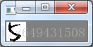

然後呼叫模型結果如下：

結果是5，預測準確。
上面的是做測試結果，關於試卷識別，我們有下面的例子，圖片如下: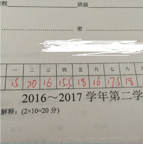

對這個圖片我們要做的是提取方框內的分數，然後識別出來數字，進行統計，最後得出分數總和，儲存起來，這就是整體思路。具體操作程式碼如下：

import numpy as np
import tensorflow as tf
import cv2
from PIL import Image
from skimage import data, util,measure,color
from skimage.measure import label
image = cv2.imread('D:\opencv_camera\digits\\12.jpg')
lower=np.array([50,50,150])
upper=np.array([140,140,250])
mask = cv2.inRange(image, lower, upper)
output1 = cv2.bitwise_and(image, image, mask=mask)

output=cv2.cvtColor(output1,cv2.COLOR_BGR2GRAY)
th2 = cv2.adaptiveThreshold(output,255,cv2.ADAPTIVE_THRESH_GAUSSIAN_C,cv2.THRESH_BINARY,11,0)
# cv2.imshow("images",th2)
# cv2.waitKey(0)
roi=[]
for i in range(8):
    img_roi = output1[260:310,35+55*i:80+58*i]
    roi.append(img_roi)

#歸一化
def normalizepic(pic):
    im_arr = pic
    im_nparr = []
    for x in im_arr:
        x=1-x/255
        im_nparr.append(x)
    im_nparr = np.array([im_nparr])
    return im_nparr

########圖片預處理##########

def weight_variable(shape):
    initial=tf.truncated_normal(shape,stddev=0.1)
    return tf.Variable(initial,dtype=tf.float32,name='weight')
def bias_variable(shape):
    initial=tf.constant(0.1,shape=shape)
    return tf.Variable(initial,dtype=tf.float32,name='biases')
def conv2d(x,W):
    return tf.nn.conv2d(x,W,strides=[1,1,1,1],padding='SAME')
def max_pool_2x2(x):
    return tf.nn.max_pool(x,ksize=[1,2,2,1],strides=[1,2,2,1],padding='SAME')

xs=tf.placeholder(tf.float32,[None,784])#輸入是一個28*28的畫素點的資料

keep_prob=tf.placeholder(tf.float32)

x_image=tf.reshape(xs,[-1,28,28,1])#xs的維度暫時不管，用-1表示，28,28表示xs的資料，1表示該資料是一個黑白照片，如果是彩色的，則寫成3
#卷積層1
W_conv1=weight_variable([5,5,1,32])#抽取一個5*5畫素，高度是32的點,每次抽出原影象的5*5的畫素點，高度從1變成32
b_conv1=bias_variable([32])
h_conv1=tf.nn.relu(conv2d(x_image,W_conv1)+b_conv1)#輸出 28*28*32的影象
h_pool1=max_pool_2x2(h_conv1)##輸出14*14*32的影象，因為這個函式的步長是2*2，影象縮小一半。
#卷積層2
W_conv2=weight_variable([5,5,32,64])#隨機生成一個5*5畫素，高度是64的點,抽出原影象的5*5的畫素點，高度從32變成64
b_conv2=bias_variable([64])
h_conv2=tf.nn.relu(conv2d(h_pool1,W_conv2)+b_conv2)#輸出14*14*64的影象
h_pool2=max_pool_2x2(h_conv2)##輸出7*7*64的影象，因為這個函式的步長是2*2，影象縮小一半。
#fully connected 1
W_fc1=weight_variable([7*7*64,1024])
b_fc1=bias_variable([1024])
h_pool2_flat=tf.reshape(h_pool2,[-1,7*7*64])#將輸出的h_pool2的三維資料變成一維資料，平鋪下來，（-1）代表的是有多少個例子
h_fc1=tf.nn.relu(tf.matmul(h_pool2_flat,W_fc1)+b_fc1)
h_fc1_drop=tf.nn.dropout(h_fc1,keep_prob)
#fully connected 2
W_fc2=weight_variable([1024,10])
b_fc2=bias_variable([10])
prediction=tf.nn.softmax(tf.matmul(h_fc1_drop,W_fc2)+b_fc2)#輸出層
with tf.Session() as sess:
    sess.run(tf.global_variables_initializer())
    saver = tf.train.Saver()
    saver.restore(sess, "my_net/save_net.ckpt")
    result= tf.argmax(prediction, 1)
    SUM=[]
    for i in range(8):
        output = cv2.cvtColor(roi[i], cv2.COLOR_BGR2GRAY)
        th2 = cv2.adaptiveThreshold(output, 255, cv2.ADAPTIVE_THRESH_GAUSSIAN_C, cv2.THRESH_BINARY, 11, 0)
        # cv2.imshow("images", th2)
        # cv2.waitKey(0)
        labels = label(th2, connectivity=2)
        dst = color.label2rgb(labels)
        a=[]
        for region in measure.regionprops(labels):
            minr, minc, maxr, maxc = region.bbox
            # img = cv2.rectangle(dst, (minc -10 , minr - 10), (maxc + 10, maxr + 10), (0, 255, 0), 1)
            ROI = th2[minr - 2:maxr + 2, minc - 2:maxc + 2]
            if ROI.shape[1] < 10:
                kernel = cv2.getStructuringElement(cv2.MORPH_RECT, (2, 2))
                ROI = cv2.erode(ROI, kernel, iterations=1)
            ret, thresh2 = cv2.threshold(ROI, 0, 255, cv2.THRESH_BINARY_INV)
            res = cv2.resize(thresh2, (28, 28), interpolation=cv2.INTER_CUBIC)
            cv2.imshow("images", res)
            cv2.waitKey(0)
            img = normalizepic(res).reshape((1, 784))
            img = img.astype(np.float32)
            result=sess.run(prediction, feed_dict={xs:img,keep_prob: 1.0})
            result1 =np.argmax(result,1)
            print(result1)
            a.append(result1)
        if len(a)==2:
            #print(a[1]*10+a[0])
            SUM.append(a[1]*10+a[0])
        else:
            #print(a[0])
            SUM.append(a[0])

print(sum(SUM))

將最後的結果儲存在列表中，得出結果。整個程式碼寫到這裡基本上就完成了，在影象處理過程中，需要掌握opencv的一些具體的操作，包括影象二值化，特定區域ROI提取，在對影象進行分割的時候用到了skimage庫，這個庫可以對不同連通區域的影象進行分割，非常方便實用。整個過程還存在一些問題需要完善，包括對於粘連的數字如何處理，之前查過一篇文獻光學手寫數字字元識別技術的研究,裡面提到了一種用水滴法分割粘連字元，整個識別過程還存在一些不足，後續還有很大的改善空間。

學習記錄：一個試卷批改系統

學習記錄：一個試卷批改系統

git原理學習記錄：從基本指令到背後原理，實現一個簡單的git

學習記錄：安裝配置自動化工具ansible

Linux 學習記錄：七、fdisk 分區工具

學習記錄：gcc/g++ 編譯與鏈接

全文搜索引擎ElasticSearch學習記錄：mac下安裝

記錄：一個SQL SERVER奇怪的問題。

JSP學習記錄：request物件

小程式學習記錄：讀取discuz生成的json資料

MyBatis 學習記錄7 一個Bug引發的思考

HTTP學習記錄：四、頭資訊（請求和響應）

Qt5學習記錄：QString與int值互相轉換

LearnOpenGL學習筆記(七):一個FPS攝像機系統

小程式學習記錄：顯示陣列內容2

Coursera 學習記錄：Tomorrow never knows？（實現日期加一的操作）

Coursera 學習記錄：四大湖排序（使用bool值的小技巧）

Coursera 學習記錄：發票統計（使用switch進行資料歸類）

Coursera 學習記錄：流感傳染（關於二維陣列的標記和統計）

R in Action學習筆記：一個簡單的資料處理例項

js學習記錄：變數，函式，事件相關

學習記錄：一個試卷批改系統

相關推薦