
Tensorflow深度學習之二十二:AlexNet的實現(CIFAR-10資料集)
二、工程結構
由於我自己訓練的機器記憶體視訊記憶體不足,不能一次性讀取10000張圖片,因此,在這之前我按照圖片的類別,將每一張圖片都提取了出來,儲存成了jpg格式。與此同時,在儲存圖片的過程中,儲存了一個python的dict結構,鍵為每一張圖片的相對地址,值為每一張圖片對應的類別,將這個dict結構儲存成npy檔案。每一張jpg圖片的大小為32*32,而AlexNet需要的輸入為224*224,所以在讀取圖片的時候需要使用cv2.resize進行圖片解析度的調整。
分別對訓練集和測試集做以上操作。得到的工程目錄如下所示:
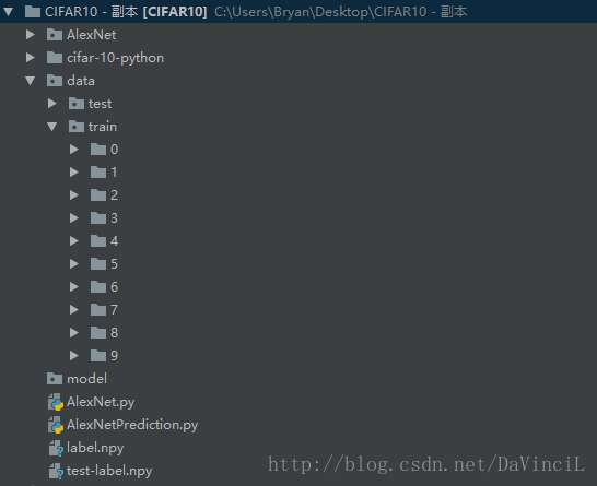
每個檔案和資料夾的作用顯示如下:
| 檔案 | 作用 |
|---|---|
| AlexNet資料夾 | 儲存相關日誌的資料夾 |
| cifar-10-python資料夾 | 儲存CIFAR-10資料集的原始檔 |
| data\test | 測試集資料 |
| data\train | 訓練集資料,按照標籤分成十類,分別儲存在0~9的資料夾內,test資料夾也是一樣 |
| model資料夾 | 儲存模型的目錄 |
| AlexNet.py | 建立AlexNet網路結構和訓練 |
| AlexNetPrediction.py | 使用訓練好的模型進行預測 |
| label.npy | 儲存訓練集的檔名與標籤的檔案,是一個dict |
| test-label.npy | 儲存測試集的檔名與標籤的檔案,是一個dict |
三,訓練程式碼
import tensorflow as tf
import numpy as np
import random
import cv2
# 將傳入的label轉換成one hot的形式。
def getOneHotLabel(label, depth):
m = np.zeros([len(label), depth])
for i in range(len(label)):
m[i][label[i]] = 1
return m
# 建立神經網路。
def alexnet(image, keepprob=0.5):
# 定義卷積層1,卷積核大小,偏置量等各項引數參考下面的程式程式碼,下同。 以下為結果的部分輸出:
50000
1.781297Epoch  0 : validation rate:  0.562699974775
1.775934Epoch  1 : validation rate:  0.547099971175
1.768913Epoch  2 : validation rate:  0.52679997623
1.719084Epoch  3 : validation rate:  0.548099977374
1.721695Epoch  4 : validation rate:  0.562299972177
1.745009Epoch  5 : validation rate:  0.56409997642
1.746290Epoch  6 : validation rate:  0.612299977541
1.726248Epoch  7 : validation rate:  0.574799978137
1.735083Epoch  8 : validation rate:  0.617399973869
1.722523Epoch  9 : validation rate:  0.61839998126
1.712282Epoch  10 : validation rate:  0.643999977112
1.697912Epoch  11 : validation rate:  0.63789998889
1.708088Epoch  12 : validation rate:  0.641699975729
1.716783Epoch  13 : validation rate:  0.64499997735
1.718689Epoch  14 : validation rate:  0.664099971056
1.712452Epoch  15 : validation rate:  0.659299976826
1.699410Epoch  16 : validation rate:  0.666799970865
1.682442Epoch  17 : validation rate:  0.660699977875
1.650028Epoch  18 : validation rate:  0.673199976683
1.662869Epoch  19 : validation rate:  0.692699990273
1.652857Epoch  20 : validation rate:  0.687699975967
1.672175Epoch  21 : validation rate:  0.710799975395
1.662848Epoch  22 : validation rate:  0.707699980736
1.653844Epoch  23 : validation rate:  0.708999979496
1.636483Epoch  24 : validation rate:  0.736199990511
1.658812Epoch  25 : validation rate:  0.688499983549
1.658808Epoch  26 : validation rate:  0.748899987936
1.642705Epoch  27 : validation rate:  0.751199992895
1.609915Epoch  28 : validation rate:  0.742099983692
1.610037Epoch  29 : validation rate:  0.757699984312
1.647516Epoch  30 : validation rate:  0.771899987459
1.615854Epoch  31 : validation rate:  0.762699997425
1.598617Epoch  32 : validation rate:  0.785299996138
1.579349Epoch  33 : validation rate:  0.791699982882
1.615915Epoch  34 : validation rate:  0.780799984932
1.586894Epoch  35 : validation rate:  0.790699990988
1.573043Epoch  36 : validation rate:  0.799299983978
1.580690Epoch  37 : validation rate:  0.812399986982
1.598764Epoch  38 : validation rate:  0.824699985981
1.566866Epoch  39 : validation rate:  0.821999987364
在實際的訓練過程中,我進行了多次訓練,每次在前一模型的基礎上調整學習率繼續進行訓練。最後的loss值可以下降到1.3~1.4,驗證集的正確率可以到0.96~0.97。
四、預測程式碼
預測程式碼:
import tensorflow as tf
import numpy as np
import random
import cv2

def getOneHotLabel(label, depth):
    m = np.zeros([len(label), depth])
    for i in range(len(label)):
        m[i][label[i]] = 1
    return m

# 建立神經網路
def alexnet(image, keepprob=0.5):

    # 定義卷積層1,卷積核大小,偏置量等各項引數參考下面的程式程式碼,下同
    with tf.name_scope("conv1") as scope:
        kernel = tf.Variable(tf.truncated_normal([11, 11, 3, 64], dtype=tf.float32, stddev=1e-1, name="weights"))
        conv = tf.nn.conv2d(image, kernel, [1, 4, 4, 1], padding="SAME")
        biases = tf.Variable(tf.constant(0.0, dtype=tf.float32, shape=[64]), trainable=True, name="biases")
        bias = tf.nn.bias_add(conv, biases)
        conv1 = tf.nn.relu(bias, name=scope)

        pass

    # LRN層
    lrn1 = tf.nn.lrn(conv1, 4, bias=1.0, alpha=0.001/9, beta=0.75, name="lrn1")

    # 最大池化層
    pool1 = tf.nn.max_pool(lrn1, ksize=[1,3,3,1], strides=[1,2,2,1],padding="VALID", name="pool1")

    # 定義卷積層2
    with tf.name_scope("conv2") as scope:
        kernel = tf.Variable(tf.truncated_normal([5,5,64,192], dtype=tf.float32, stddev=1e-1, name="weights"))
        conv = tf.nn.conv2d(pool1, kernel, [1, 1, 1, 1], padding="SAME")
        biases = tf.Variable(tf.constant(0.0, dtype=tf.float32, shape=[192]), trainable=True, name="biases")
        bias = tf.nn.bias_add(conv, biases)
        conv2 = tf.nn.relu(bias, name=scope)
        pass

    # LRN層
    lrn2 = tf.nn.lrn(conv2, 4, bias=1.0, alpha=0.001 / 9, beta=0.75, name="lrn2")

    # 最大池化層
    pool2 = tf.nn.max_pool(lrn2, ksize=[1, 3, 3, 1], strides=[1, 2, 2, 1], padding="VALID", name="pool2")

    # 定義卷積層3
    with tf.name_scope("conv3") as scope:
        kernel = tf.Variable(tf.truncated_normal([3,3,192,384], dtype=tf.float32, stddev=1e-1, name="weights"))
        conv = tf.nn.conv2d(pool2, kernel, [1, 1, 1, 1], padding="SAME")
        biases = tf.Variable(tf.constant(0.0, dtype=tf.float32, shape=[384]), trainable=True, name="biases")
        bias = tf.nn.bias_add(conv, biases)
        conv3 = tf.nn.relu(bias, name=scope)
        pass

    # 定義卷積層4
    with tf.name_scope("conv4") as scope:
        kernel = tf.Variable(tf.truncated_normal([3,3,384,256], dtype=tf.float32, stddev=1e-1, name="weights"))
        conv = tf.nn.conv2d(conv3, kernel, [1, 1, 1, 1], padding="SAME")
        biases = tf.Variable(tf.constant(0.0, dtype=tf.float32, shape=[256]), trainable=True, name="biases")
        bias = tf.nn.bias_add(conv, biases)
        conv4 = tf.nn.relu(bias, name=scope)
        pass

    # 定義卷積層5
    with tf.name_scope("conv5") as scope:
        kernel = tf.Variable(tf.truncated_normal([3,3,256,256], dtype=tf.float32, stddev=1e-1, name="weights"))
        conv = tf.nn.conv2d(conv4, kernel, [1, 1, 1, 1], padding="SAME")
        biases = tf.Variable(tf.constant(0.0, dtype=tf.float32, shape=[256]), trainable=True, name="biases")
        bias = tf.nn.bias_add(conv, biases)
        conv5 = tf.nn.relu(bias, name=scope)
        pass

    # 最大池化層
    pool5 = tf.nn.max_pool(conv5, ksize=[1,3,3,1], strides=[1,2,2,1], padding="VALID", name="pool5")

    # 全連線層
    flatten = tf.reshape(pool5, [-1, 6*6*256])

    weight1 = tf.Variable(tf.truncated_normal([6*6*256, 4096], mean=0, stddev=0.01))

    fc1 = tf.nn.sigmoid(tf.matmul(flatten, weight1))

    dropout1 = tf.nn.dropout(fc1, keepprob)

    weight2 = tf.Variable(tf.truncated_normal([4096, 4096], mean=0, stddev=0.01))

    fc2 = tf.nn.sigmoid(tf.matmul(dropout1, weight2))

    dropout2 = tf.nn.dropout(fc2, keepprob)

    weight3 = tf.Variable(tf.truncated_normal([4096, 10], mean=0, stddev=0.01))

    fc3 = tf.nn.sigmoid(tf.matmul(dropout2, weight3))

    return fc3


def alexnet_main():
    # 載入測試集的檔名和標籤。
    files = np.load("test-label.npy", encoding='bytes')[()]
    keys = [i for i in files]
    print(len(keys))

    myinput = tf.placeholder(dtype=tf.float32, shape=[None, 224, 224, 3], name='input')
    mylabel = tf.placeholder(dtype=tf.float32, shape=[None, 10], name='label')
    myoutput = alexnet(myinput, 0.6)

    prediction = tf.argmax(myoutput, 1)
    truth = tf.argmax(mylabel, 1)
    valaccuracy = tf.reduce_mean(
        tf.cast(
            tf.equal(
                prediction,
                truth),
            tf.float32))

    saver = tf.train.Saver()

    with tf.Session() as sess:
        # 載入訓練好的模型,路徑根據自己的實際情況調整
        saver.restore(sess, r"model/model.ckpt")

        cnt = 0
        for i in range(10000):
            photo = []
            label = []

            photo.append(cv2.resize(cv2.imread(keys[i]), (224, 224))/225)
            label.append(files[keys[i]])
            m = getOneHotLabel(label, depth=10)
            a, b= sess.run([prediction, truth], feed_dict={myinput: photo, mylabel: m})
            print(a, ' ', b)
            if a[0] == b[0]:
                cnt += 1

        print("Epoch ", 1, ': prediction rate: ', cnt / 10000)

if __name__ == '__main__':
    alexnet_main()
預測結果:(這裡只顯示部分輸出結果)
10000
[3]   [3]
[8]   [8]
[6]   [6]
[4]   [4]
[5]   [9]
[2]   [3]
[9]   [9]
[5]   [5]
[1]   [7]
[3]   [4]
[4]   [4]
[4]   [3]
[9]   [9]
[5]   [5]
[8]   [8]
[3]   [8]
[0]   [0]
[8]   [8]
[7]   [7]
[7]   [4]
[7]   [7]
[5]   [5]
[6]   [5]
...
[7]   [7]
[3]   [3]
[0]   [0]
[7]   [4]
[6]   [2]
[0]   [0]
[7]   [7]
[2]   [5]
[8]   [8]
[5]   [3]
[5]   [5]
[1]   [1]
[7]   [7]
Epoch  1 : prediction rate:  0.7685
五、結果分析
在測試集的表現上,自己訓練的AlexNet網路的預測結果達到了0.7685,即76.85%的正確率。相比較LeNet,這個結果好很多,這是因為在網路結構中,使用了更多的卷積操作,可以提取更多的潛在特徵。足以證明AlexNet在CIFAR-10資料集上表現比LeNet好。
但是0.7685的正確率還是不是很讓人滿意,所以後面可以選擇繼續調整網路的引數,調整網路的結構等手段繼續進行網路的訓練,或者可以選擇使用預訓練好的模型進行自己網路的訓練,或者可以嘗試使用其他更加優秀的網路結構。
接下來的任務是嘗試使用GoogleNet模型進行CIFAR-10資料集的求解。
2018年6月13日更新
很多朋友在評論區問我兩個npy檔案怎麼生成的,其實我就是把所有的圖片都儲存下來,然後把資訊提取出來,儲存了一下而已。下面是提取資訊和儲存的程式碼,非常簡單。
import numpy as np
import os


train_label = {}

for i in range(10):
    search_path = './data/train/{}'.format(i)
    file_list = os.listdir(search_path)
    for file in file_list:
        train_label[os.path.join(search_path, file)] = i

np.save('label.npy', train_label)

test_label = {}

for i in range(10):
    search_path = './data/test/{}'.format(i)
    file_list = os.listdir(search_path)
    for file in file_list:
        test_label[os.path.join(search_path, file)] = i

np.save('test-label.npy', test_label)
如果目錄結構和上面的是一樣的話,把這些程式碼檔案放在工程的根目錄下面就可以執行,也可以根據自己需要調整,目的可以達到就可以了。