《利用python做資料分析》第十章:時間序列分析
阿新 • • 發佈:2019-01-24
import pandas as pd
import numpy as np
import matplotlib.pyplot as plt
%matplotlib inlinefrom from datetime import datetimenow = datetime.now()now(2016, 2, 1) datetime以毫秒形勢儲存��和⌚️,**datetime.datedelta**表示兩個datetime物件之間的時間差now.year,now.month,now.day
delta = datetime(2011,1,7) - datetime(2008,6,24,8,15)deltafrom start = datetime(2011, 1, 7)start + timedelta(12)start - timedelta(12) * 4stamp = datetime(2011, 1, 3)str(stamp)stamp.strftime('%Y-%m-%d')stamp.strftime('%Y-%m')value = '2011-01-03'datetime.strptime(value, '%Y-%m-%d')datestrs = ['7/6/2011','8/6/2011'][datetime.strptime(x, '%m/%d/%Y') for x in datestrs]from dateutil.parser import parseparse('2011-01-03')parse('Jan 31,1997 10:45 PM')parse('6/30/2011', dayfirst=True)datestrspd.to_datetime(datestrs)dates = [datetime(2011, 1, 2),datetime(2011,1,5),datetime(2011,1,7),
datetime(2011,1,8),datetime(2011,1,10),datetime(2011,1,12)]ts = Series(np.random.randn(6), index=dates)tstype(ts)ts.indexts + ts[::2]ts[::2]ts['1/10/2011']ts['20110110']longer_ts=Series(np.random.randn(1000),index=pd.date_range('20000101',periods=1000))longer_tslonger_ts['2002']longer_ts['2001/03']ts['20110101':'20110201']ts.truncate(after='20110109')dates = pd.date_range('20000101', periods=100, freq='W-WED')dateslong_df = DataFrame(np.random.randn(100,4),index=dates,columns=['Colorado','Texas','New York','Ohio'])long_df.ix['5-2001']| Colorado | Texas | New York | Ohio | |
|---|---|---|---|---|
| 2001-05-02 | 1.783070 | 1.090816 | -1.035363 | -0.089864 |
| 2001-05-09 | -1.290700 | 1.311863 | -0.596037 | 0.819694 |
| 2001-05-16 | 0.688693 | -0.249644 | -0.859212 | 0.879270 |
| 2001-05-23 | -1.602660 | 1.211236 | -1.028336 | 2.022514 |
| 2001-05-30 | -0.705427 | -0.189235 | -0.710712 | -2.397815 |
dates = pd.DatetimeIndex(['1/1/2000','1/2/2000',
                         '1/2/2000','1/2/2000',
                         '1/3/2000'])
dup_ts = Series(np.arange(5), index=dates)dup_tsdup_ts.index.is_uniquedup_ts['1/3/2000']dup_ts['1/2/2000']dup_ts.index.is_uniquegrouped = dup_ts.groupby(level=0)grouped.mean(),grouped.count()ts.resample('D')index = pd.date_range('4/1/2012','6/1/2012')from pandas.tseries.offsets import Hour, Minutehour = Hour()hourfour_hours = Hour(4)four_hourspd.date_range('1/1/2000','1/3/2000 23:59',freq='4h')Hour(2) + Minute(30)pd.date_range('1/1/2000', periods=10, freq='1h30min')rng = pd.date_range('1/1/2012','9/1/2012',freq='WOM-3FRI')pd.date_range('1/1/2012','9/1/2012',freq='W-FRI')ts = Series(np.random.randn(4),index=pd.date_range('1/1/2000',periods=4,freq='M'))tsts.shift(-2)ts / ts.shift(1) - 1ts.pct_change()ts.shift(2, freq='M')ts.shift(3, freq='D')type(ts)ts.shift()ts.shift(3)ts.shift(freq='D')ts.shift(periods=2)from pandas.tseries.offsets import Day, MonthEndnow = datetime(2011, 11, 17)now + 3*Day()now + MonthEnd()now + MonthEnd(2)offset = MonthEnd()offset.rollforward(now)offset.rollback(now)ts = Series(np.random.randn(20), index=pd.date_range('1/15/2000',periods=20,freq='4d'))ts.groupby(offset.rollforward).mean()ts.resample('M', how='mean')import pytzpytz.common_timezones[-5:]tz = pytz.timezone('US/Eastern')tzrng = pd.date_range('3/9/2012 9:30',periods=6, freq='D')
ts = Series(np.random.randn(len(rng)),index=rng)del indexts.index.tzpd.date_range('3/9/2000 9:30',periods=10, freq='D',tz='UTC')ts_utc = ts.tz_localize('UTC')
ts_utcts_utc.indexts_utc.tz_convert('US/Eastern')ts.index.tz_localize('Asia/Shanghai')stamp = pd.Timestamp('2011-03-12 4:00')
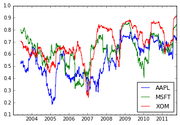
stamp_utc = stamp.tz_localize('utc')stamp_utc.tz_convert('US/Eastern')stamp_utc.valuestamp = pd.Timestamp('2012-03-12 01:30', tz='US/Eastern')stampstamp + Hour()rng = pd.date_range('3/7/2012 9:30',periods=10, freq='B')ts = Series(np.random.randn(len(rng)), index=rng)tsts1 = ts[:7].tz_localize('Europe/London')ts2 = ts1[2:].tz_convert('Europe/Moscow')result = ts1 + ts2result.indexp = pd.Period(2007, freq='A-DEC')pclose_px_call = pd.read_csv('/Users/Houbowei/Desktop/SRP/books/pydata-book-master/pydata-book-master/ch09/stock_px.csv', parse_dates=True,index_col=0)close_px = close_px_call[['AAPL','MSFT','XOM']]close_px = close_px.resample('B',fill_method='ffill')close_px| AAPL | MSFT | XOM | |
|---|---|---|---|
| 2003-01-02 | 7.40 | 21.11 | 29.22 |
| 2003-01-03 | 7.45 | 21.14 | 29.24 |
| 2003-01-06 | 7.45 | 21.52 | 29.96 |
| 2003-01-07 | 7.43 | 21.93 | 28.95 |
| 2003-01-08 | 7.28 | 21.31 | 28.83 |
| 2003-01-09 | 7.34 | 21.93 | 29.44 |
| 2003-01-10 | 7.36 | 21.97 | 29.03 |
| 2003-01-13 | 7.32 | 22.16 | 28.91 |
| 2003-01-14 | 7.30 | 22.39 | 29.17 |
| 2003-01-15 | 7.22 | 22.11 | 28.77 |
| 2003-01-16 | 7.31 | 21.75 | 28.90 |
| 2003-01-17 | 7.05 | 20.22 | 28.60 |
| 2003-01-20 | 7.05 | 20.22 | 28.60 |
| 2003-01-21 | 7.01 | 20.17 | 27.94 |
| 2003-01-22 | 6.94 | 20.04 | 27.58 |
| 2003-01-23 | 7.09 | 20.54 | 27.52 |
| 2003-01-24 | 6.90 | 19.59 | 26.93 |
| 2003-01-27 | 7.07 | 19.32 | 26.21 |
| 2003-01-28 | 7.29 | 19.18 | 26.90 |
| 2003-01-29 | 7.47 | 19.61 | 27.88 |
| 2003-01-30 | 7.16 | 18.95 | 27.37 |
| 2003-01-31 | 7.18 | 18.65 | 28.13 |
| 2003-02-03 | 7.33 | 19.08 | 28.52 |
| 2003-02-04 | 7.30 | 18.59 | 28.52 |
| 2003-02-05 | 7.22 | 18.45 | 28.11 |
| 2003-02-06 | 7.22 | 18.63 | 27.87 |
| 2003-02-07 | 7.07 | 18.30 | 27.66 |
| 2003-02-10 | 7.18 | 18.62 | 27.87 |
| 2003-02-11 | 7.18 | 18.25 | 27.67 |
| 2003-02-12 | 7.20 | 18.25 | 27.12 |
| … | … | … | … |
| 2011-09-05 | 374.05 | 25.80 | 72.14 |
| 2011-09-06 | 379.74 | 25.51 | 71.15 |
| 2011-09-07 | 383.93 | 26.00 | 73.65 |
| 2011-09-08 | 384.14 | 26.22 | 72.82 |
| 2011-09-09 | 377.48 | 25.74 | 71.01 |
| 2011-09-12 | 379.94 | 25.89 | 71.84 |
| 2011-09-13 | 384.62 | 26.04 | 71.65 |
| 2011-09-14 | 389.30 | 26.50 | 72.64 |
| 2011-09-15 | 392.96 | 26.99 | 74.01 |
| 2011-09-16 | 400.50 | 27.12 | 74.55 |
| 2011-09-19 | 411.63 | 27.21 | 73.70 |
| 2011-09-20 | 413.45 | 26.98 | 74.01 |
| 2011-09-21 | 412.14 | 25.99 | 71.97 |
| 2011-09-22 | 401.82 | 25.06 | 69.24 |
| 2011-09-23 | 404.30 | 25.06 | 69.31 |
| 2011-09-26 | 403.17 | 25.44 | 71.72 |
| 2011-09-27 | 399.26 | 25.67 | 72.91 |
| 2011-09-28 | 397.01 | 25.58 | 72.07 |
| 2011-09-29 | 390.57 | 25.45 | 73.88 |
| 2011-09-30 | 381.32 | 24.89 | 72.63 |
| 2011-10-03 | 374.60 | 24.53 | 71.15 |
| 2011-10-04 | 372.50 | 25.34 | 72.83 |
| 2011-10-05 | 378.25 | 25.89 | 73.95 |
| 2011-10-06 | 377.37 | 26.34 | 73.89 |
| 2011-10-07 | 369.80 | 26.25 | 73.56 |
| 2011-10-10 | 388.81 | 26.94 | 76.28 |
| 2011-10-11 | 400.29 | 27.00 | 76.27 |
| 2011-10-12 | 402.19 | 26.96 | 77.16 |
| 2011-10-13 | 408.43 | 27.18 | 76.37 |
| 2011-10-14 | 422.00 | 27.27 | 78.11 |
2292 rows × 3 columns
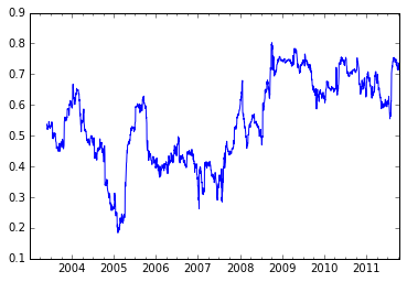
close_px.resample?close_px['AAPL'].plot()close_px.ix['2009'].plot()close_px['AAPL'].ix['01-2011':'03-2011'].plot()apple_q = close_px['AAPL'].resample('Q-DEC', fill_method='ffill')apple_q.ix['2009':].plot()close_px.AAPL.plot()close_px.plot()apple_std250 = pd.rolling_std(close_px.AAPL, 250)apple_std250.describe()apple_std250.plot()close_px.describe()| AAPL | MSFT | XOM | |
|---|---|---|---|
| count | 2292.000000 | 2292.000000 | 2292.000000 |
| mean | 125.339895 | 23.953010 | 59.568473 |
| std | 107.218553 | 3.267322 | 16.731836 |
| min | 6.560000 | 14.330000 | 26.210000 |
| 25% | 37.122500 | 21.690000 | 49.517500 |
| 50% | 91.365000 | 24.000000 | 62.980000 |
| 75% | 185.535000 | 26.280000 | 72.540000 |
| max | 422.000000 | 34.070000 | 87.480000 |
close_px_call.describe()| AAPL | MSFT | XOM | SPX | |
|---|---|---|---|---|
| count | 2214.000000 | 2214.000000 | 2214.000000 | 2214.000000 |
| mean | 125.516147 | 23.945452 | 59.558744 | 1183.773311 |
| std | 107.394693 | 3.255198 | 16.725025 | 180.983466 |
| min | 6.560000 | 14.330000 | 26.210000 | 676.530000 |
| 25% | 37.135000 | 21.700000 | 49.492500 | 1077.060000 |
| 50% | 91.455000 | 24.000000 | 62.970000 | 1189.260000 |
| 75% | 185.605000 | 26.280000 | 72.510000 | 1306.057500 |
| max | 422.000000 | 34.070000 | 87.480000 | 1565.150000 |
spx = close_px_call.SPX.pct_change()spx2003-01-02 NaN
2003-01-03 -0.000484
2003-01-06 0.022474
2003-01-07 -0.006545
2003-01-08 -0.014086
2003-01-09 0.019386
2003-01-10 0.000000
2003-01-13 -0.001412
2003-01-14 0.005830
2003-01-15 -0.014426
2003-01-16 -0.003942
2003-01-17 -0.014017
2003-01-21 -0.015702
2003-01-22 -0.010432
2003-01-23 0.010224
2003-01-24 -0.029233
2003-01-27 -0.016160
2003-01-28 0.013050
2003-01-29 0.006779
2003-01-30 -0.022849
2003-01-31 0.013130
2003-02-03 0.005399
2003-02-04 -0.014088
2003-02-05 -0.005435
2003-02-06 -0.006449
2003-02-07 -0.010094
2003-02-10 0.007569
2003-02-11 -0.008098
2003-02-12 -0.012687
2003-02-13 -0.001600
...
2011-09-02 -0.025282
2011-09-06 -0.007436
2011-09-07 0.028646
2011-09-08 -0.010612
2011-09-09 -0.026705
2011-09-12 0.006966
2011-09-13 0.009120
2011-09-14 0.013480
2011-09-15 0.017187
2011-09-16 0.005707
2011-09-19 -0.009803
2011-09-20 -0.001661
2011-09-21 -0.029390
2011-09-22 -0.031883
2011-09-23 0.006082
2011-09-26 0.023336
2011-09-27 0.010688
2011-09-28 -0.020691
2011-09-29 0.008114
2011-09-30 -0.024974
2011-10-03 -0.028451
2011-10-04 0.022488
2011-10-05 0.017866
2011-10-06 0.018304
2011-10-07 -0.008163
2011-10-10 0.034125
2011-10-11 0.000544
2011-10-12 0.009795
2011-10-13 -0.002974
2011-10-14 0.017380
Name: SPX, dtype: float64
returns = close_px.pct_change()corr = pd.rolling_corr(returns.AAPL, spx, 125 , min_periods=100)corr.plot()<matplotlib.axes._subplots.AxesSubplot at 0x10bf49450>
corr = pd.rolling_corr(returns, spx, 125, min_periods=100).plot()