
利用R語言預測銀行客戶信用的優劣(隨機森林方法)
我們選取的資料時1994年德國的一家銀行在平定客戶信用風險好壞的時候用到的一組變數,共有1000組資料。由於年代久遠可能和實際有些出入。資料可以在下面的網址下載。 http://archive.ics.uci.edu/ml/datasets/Statlog+(German+Credit+Data)
主要提供了兩組資料,一份是原始資料總共有20個變數,另一分時處理過的數值資料,為了尋求更深層次的資料探勘我們將分別利用者兩組資料。
我們首先簡單介紹一下變數
變數1
Status of existing checking account 現有的支票賬戶狀態
A11 : … < 0 DM
A12 : 0 <= … < 200 DM
A13 : … >= 200 DM / salary assignments for at least 1 year
A14 : no checking account
變數2: (numerical) 數值變數(這裡應該表示的是貸款期限)
Duration in month 月持續時間
變數3: (qualitative) 質量變數信用歷史
Credit history 信用記錄
A30 : no credits taken/ all credits paid back duly 無信用記錄或所有信用都及時償還
A31 : all credits at this bank paid back duly 這家銀行的所有信用都及時償還
A32 : existing credits paid back duly till now 直到現在有信用及時償還
A33 : delay in paying off in the past 過去存在延遲支付
A34 : critical account/ other credits existing (not at this bank) 關鍵賬戶/在其他銀行存在信用記錄
變數4: (qualitative) 質量變數
Purpose 貸款目的
A40 : car (new) 新車
A41 : car (used) 舊車
A42 : furniture/equipment 傢俱/裝置
A43 : radio/television 收音機/電視
A44 : domestic appliances 家用電器
A45 : repairs 維修
A46 : education 教育
A47 : (vacation - does not exist ) 空白—不存在
A48 : retraining 再教育
A49 : business 商業
A410 : others 其他
變數5: (numerical) 數值變數
Credit amount 信貸額度
Attibute 6: (qualitative) 質量變數
Savings account/bonds 存款
A61 : … < 100 DM
A62 : 100 <= … < 500 DM
A63 : 500 <= … < 1000 DM
A64 : .. >= 1000 DM
A65 : unknown/ no savings account 未知/無存款
變數7: (qualitative) 質量變數
Present employment since 就業狀態
A71 : unemployed 失業
A72 : … < 1 year
A73 : 1 <= … < 4 years
A74 : 4 <= … < 7 years
A75 : .. >= 7 years
變數8: (numerical) 數值變數
Installment rate in percentage of disposable income 分期費率在可支配收入的百分比
變數9: (qualitative)
Personal status and sex 個人狀態和性別
A91 : male : divorced/separated 男/離異/分居
A92 : female : divorced/separated/married 女/離異/分居/已婚
A93 : male : single 男/單身
A94 : male : married/widowed 男/已婚/喪偶
A95 : female : single 女/單身
變數10: (qualitative) 質量變數
Other debtors / guarantors 其他債務/擔保
A101 : none 無
A102 : co-applicant 共同申請人
A103 : guarantor 擔保人
變數11: (numerical)
Present residence since 目前自住宅
變數12: (qualitative)
Property 財產
A121 : real estate 房產
A122 : if not A121 : building society savings agreement/ life insurance 儲蓄/壽險
A123 : if not A121/A122 : car or other, not in 變數6 汽車或其他不在6之內
A124 : unknown / no property 未知/無財產
變數13: (numerical)
Age in years 足歲年齡
變數14: (qualitative)
Other installment plans 其他分期付款計劃
A141 : bank 銀行
A142 : stores 商店
A143 : none 無
變數15: (qualitative)
Housing
A151 : rent 租房
A152 : own 自有
A153 : for free 免租
變數16: (numerical)
Number of existing credits at this bank 在本銀行現有的信貸數量
變數17: (qualitative)
Job 工作
A171 : unemployed/ unskilled - non-resident 失業/無技能—非定居者
A172 : unskilled - resident 無技能/定居者
A173 : skilled employee / official 有技能的員工/公務員
A174 : management/ self-employed/ 管理者/個體
highly qualified employee/ officer 有經驗的員工/高階職員
變數18: (numerical)
Number of people being liable to provide maintenance for 供養人數
變數19: (qualitative)
Telephone 手機
A191 : none
A192 : yes, registered under the customers name
變數20: (qualitative)
foreign worker 外籍勞工
A201 : yes
A202 : no
最後一個變數ctedit是判斷客戶的信用優劣,1代表good,2代表bad
> germen<- read.table("C:\\Users\\Administrator\\Desktop\\german.data",header=F)
> germen@names<-c('Status','Duration','history','Purpose','Creditamount','bonds','employment','Installmentrate','Personal','guarantors','residence','Property','Age','plans','Housing','existing','Job','provide' 我們可以很清楚的看到所有的數值變數都被讀取為數值型別,所有的質量變數都被讀取為因子型別,這就是R語言的強大之處,但是這個功能也有一個弊端,比如有時一個全是數值型別的變數中不小心混入一個質量變數,R讀取時會自動認為是因子型別,為處理資料帶來麻煩。
> library(randomForest) pre.forest 1 2
1 184 65
2 14 37> table<-table(pre.forest,test$credit)
> sum(diag(table))/sum(table)
[1] 0.736我們可以看到隨機森林模型可以識別出73.6%的客戶的信用
下面我們處理這組資料,看看每個變數在建模時的重要性,以下結果僅供參考
> model.forest.all <-randomForest(credit ~ ., data =germen,importance=TRUE,proximity=TRUE)
> importance(model.forest.all)
> varImpPlot(model.forest.all)
MeanDecreaseAccuracy描述的是當把一個變數變成隨機數時,隨機森林預測準確度的降低程度,該值越大表示該變數的重要性越大。MeanDecreaseGini通過基尼指數計算每個變數對分類樹上每個節點的觀測值的異質性影響。該值越大表示該變數的重要性越大。
結果表明:個人賬戶狀態、貸款期限和信用歷史對客戶信用的優劣評判有顯著性影響。
接下來嘗試對模型進行優化
> print(model.forest)Call:
randomForest(formula = credit ~ ., data = train, importance = TRUE, proximity = TRUE)
Type of random forest: classification
Number of trees: 500
No. of variables tried at each split: 4
OOB estimate of error rate: 25.29%
Confusion matrix:
1 2 class.error
1 433 43 0.09033613構建隨機森林時,影響隨機森林模型的兩個主要因素,第一個是決策樹節點分支所選擇的變數個數,第二個是隨機森林模型中的決策數的數量,使用函式randomForest()時,函式會預設節點所選變數個數以及決策樹的數量,但是這些預設值不一定是最優的,從以上結果我們看到預設節點個數為4,決策樹的數量為500.根據這個理論。下面我們尋找最優的隨機森林模型
首先我們視覺化分析構建隨機森林模型過程中應該使用的決策樹的數量
set.seed(113)
plot(model.forest)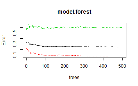
我們看到模型中的決策樹數量在200之上時都會趨於穩定,很少會有變化
接下來確定節點的個數
> for(i in 1:ncol(germen)/2)
+ {
+   set.seed(112)
+   model.forest <-randomForest(credit ~ ., data = train,mtry=i,importance=TRUE,ntree=500)
+   rate[i]=mean(model.forest$err.rate)#計算基於OOB資料的模型誤判率均值
+ }
> rate[1] 0.3499489 0.3499489 0.3291650 0.3291650 0.2997151 0.2997151 0.3032256 0.3032256 0.3073632
[10] 0.3073632plot(rate)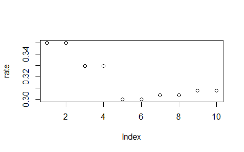
我們看到當節點為5的時候達到最小值
我們利用優化後的模型再次測試測試集,看看效果
> set.seed(114)
> model.forest1 <-randomForest(credit ~ ., data = train,mtry=5,ntree=200,importance=TRUE)
> print(model.forest1)

Call:
 randomForest(formula = credit ~ ., data = train, mtry = 5, ntree = 200,      importance = TRUE)
               Type of random forest: classification
                     Number of trees: 200
No. of variables tried at each split: 5

        OOB estimate of  error rate: 25.86%
Confusion matrix:
    1   2 class.error
1 419  57   0.1197479
2 124 100   0.5535714
> pre.forest=predict(model.forest1, test)
> table(pre.forest,test$credit)

pre.forest   1   2
         1 201  41
         2  23  35
> table<-table(pre.forest,test$credit)
> sum(diag(table))/sum(table)
[1] 0.7866667
效果還是有的由原先的0.736提高到現在的0.786.
這篇博文討論了用神經網路的方法解決銀行信用評估問題,基本思想也是將資料的70%作為一個訓練集訓練出一個神經元,之後再測試模型的好壞,正確率大約是76%。個人覺得隨機森林的最大優點是不僅能預測還可以得出每個變數的重要性,這對於建模者來說是很有意義的,尤其在商業資料探勘時,找出最重要的變數就可以為企業創造無限價值。