
Spark MLlib Linear Regression線性迴歸演算法
1、Spark MLlib Linear Regression線性迴歸演算法
1.1 線性迴歸演算法
1.1.1 基礎理論
在統計學中,線性迴歸(Linear Regression)是利用稱為線性迴歸方程的最小平方函式對一個或多個自變數和因變數之間關係進行建模的一種迴歸分析。這種函式是一個或多個稱為迴歸係數的模型引數的線性組合。
迴歸分析中,只包括一個自變數和一個因變數,且二者的關係可用一條直線近似表示,這種迴歸分析稱為一元線性迴歸分析。如果迴歸分析中包括兩個或兩個以上的自變數,且因變數和自變數之間是線性關係,則稱為多元線性迴歸分析。
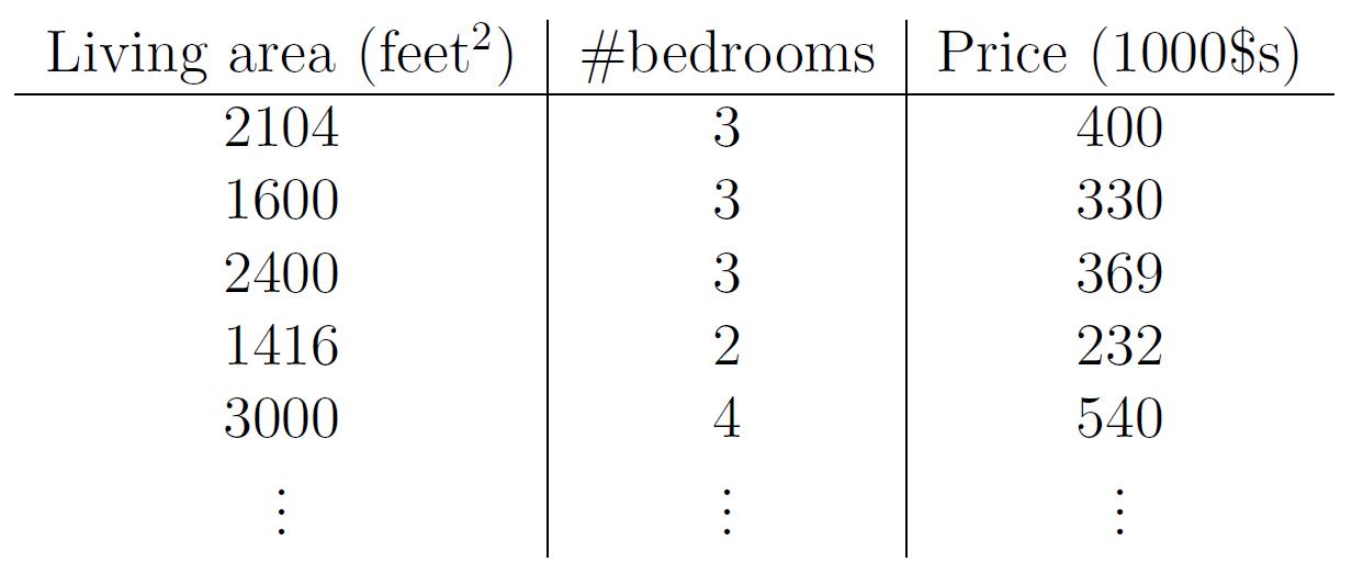
下面我們來舉例何為一元線性迴歸分析,為某地區的房屋面積(feet)
分析得到的線性方程應如下所示:

因此,無論是一元線性方程還是多元線性方程,可統一寫成如下的格式:
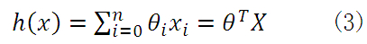
上式中x0=1,而求線性方程則演變成了求方程的引數ΘT。
線性迴歸假設特徵和結果滿足線性關係。其實線性關係的表達能力非常強大,每個特徵對結果的影響強弱可以有前面的引數體現,而且每個特徵變數可以首先對映到一個函式,然後再參與線性計算,這樣就可以表達特徵與結果之間的非線性關係。
1.1.2 梯度下降演算法
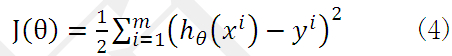
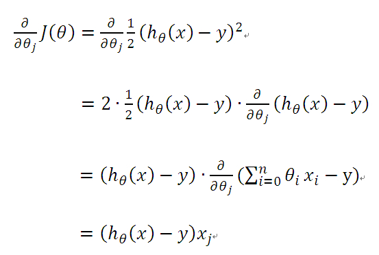
為了得到目標線性方程,我們只需確定公式(3)中的ΘT,同時為了確定所選定的的ΘT效果好壞,通常情況下,我們使用一個損失函式(loss function)或者說是錯誤函式(error function)來評估h(x)函式的好壞。該錯誤函式如公式(4)所示。前面乘上的1/2是為了在求導的時候,這個係數就不見了。
如何調整ΘT以使得J(Θ)取得最小值有很多方法,其中有完全用數學描述的最小二乘法(min square)和梯度下降法。
1.1.3 批量梯度下降演算法
由之前所述,求ΘT的問題演變成了求J(Θ)的極小值問題,這裡使用梯度下降法。而梯度下降法中的梯度方向由J(Θ)對Θ的偏導數確定,由於求的是極小值,因此梯度方向是偏導數的反方向。
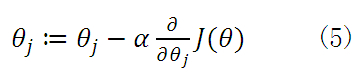
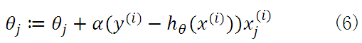
公式(5)中α為學習速率,當α過大時,有可能越過最小值,而α當過小時,容易造成迭代次數較多,收斂速度較慢。假如資料集中只有一條樣本,那麼樣本數量,所以公式(5)中
所以公式(5)就演變成:
當樣本數量m不為1時,將公式(5)中
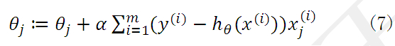
初始時ΘT可設為0,然後迭代使用公式(7)計算ΘT中的每個引數,直至收斂為止。由於每次迭代計算ΘT時,都使用了整個樣本集,因此我們稱該梯度下降演算法為批量梯度下降演算法(batch gradient descent)。
1.1.4 隨機梯度下降演算法
當樣本集資料量m很大時,批量梯度下降演算法每迭代一次的複雜度為O(mn),複雜度很高。因此,為了減少複雜度,當m很大時,我們更多時候使用隨機梯度下降演算法(stochastic gradient descent),演算法如下所示:
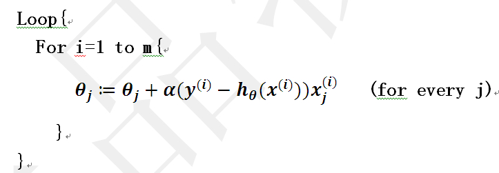
即每讀取一條樣本,就迭代對ΘT進行更新,然後判斷其是否收斂,若沒收斂,則繼續讀取樣本進行處理,如果所有樣本都讀取完畢了,則迴圈重新從頭開始讀取樣本進行處理。
這樣迭代一次的演算法複雜度為O(n)。對於大資料集,很有可能只需讀取一小部分資料,函式J(Θ)就收斂了。比如樣本集資料量為100萬,有可能讀取幾千條或幾萬條時,函式就達到了收斂值。所以當資料量很大時,更傾向於選擇隨機梯度下降演算法。
但是,相較於批量梯度下降演算法而言,隨機梯度下降演算法使得J(Θ)趨近於最小值的速度更快,但是有可能造成永遠不可能收斂於最小值,有可能一直會在最小值周圍震盪,但是實踐中,大部分值都能夠接近於最小值,效果也都還不錯。
1.1.4 最小二乘法
將訓練特徵表示為X矩陣,結果表示成y向量,仍然是線性迴歸模型,誤差函式不變。那麼θ可以直接由下面公式得出
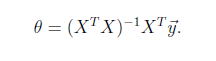
但此方法要求X是列滿秩的,而且求矩陣的逆比較慢。
1.2 Spark Mllib Linear Regression原始碼分析
1.2.1 LinearRegressionWithSGD
線性迴歸演算法的train方法,由LinearRegressionWithSGD類的object定義了train函式。
package org.apache.spark.mllib.regression
def train(
input: RDD[LabeledPoint],
numIterations: Int,
stepSize: Double,
miniBatchFraction: Double): LinearRegressionModel = {
new LinearRegressionWithSGD(stepSize, numIterations, miniBatchFraction).run(input)
}
Input為輸入樣本,numIterations為迭代次數,stepSize為步長,miniBatchFraction為迭代因子。
建立一個LinearRegressionWithSGD物件,初始化梯度下降演算法。
Run方法來自於繼承父類GeneralizedLinearAlgorithm,實現方法如下。
1.2.2 GeneralizedLinearAlgorithm
LinearRegressionWithSGD中run方法的實現。
package org.apache.spark.mllib.regression
/**
* Run the algorithm with the configured parameters on an input RDD
* of LabeledPoint entries starting from the initial weights provided.
*/
def run(input: RDD[LabeledPoint], initialWeights: Vector): M = {
// 特徵維度賦值。
if (numFeatures < 0) {
numFeatures = input.map(_.features.size).first()
}
// 輸入樣本資料檢測。
if (input.getStorageLevel == StorageLevel.NONE) {
logWarning("The input data is not directly cached, which may hurt performance if its"
+ " parent RDDs are also uncached.")
}
// 輸入樣本資料檢測。
// Check the data properties before running the optimizer
if (validateData && !validators.forall(func => func(input))) {
thrownew SparkException("Input validation failed.")
}
val scaler = if (useFeatureScaling) {
new StandardScaler(withStd = true, withMean = false).fit(input.map(_.features))
} else {
null
}
// 輸入樣本資料處理,輸出data(label, features)格式。
// addIntercept:是否增加θ0常數項,若增加,則增加x0=1項。
// Prepend an extra variable consisting of all 1.0's for the intercept.
// TODO: Apply feature scaling to the weight vector instead of input data.
val data =
if (addIntercept) {
if (useFeatureScaling) {
input.map(lp => (lp.label, appendBias(scaler.transform(lp.features)))).cache()
} else {
input.map(lp => (lp.label, appendBias(lp.features))).cache()
}
} else {
if (useFeatureScaling) {
input.map(lp => (lp.label, scaler.transform(lp.features))).cache()
} else {
input.map(lp => (lp.label, lp.features))
}
}
//初始化權重。
// addIntercept:是否增加θ0常數項,若增加,則權重增加θ0。
/**
* TODO: For better convergence, in logistic regression, the intercepts should be computed
* from the prior probability distribution of the outcomes; for linear regression,
* the intercept should be set as the average of response.
*/
val initialWeightsWithIntercept = if (addIntercept && numOfLinearPredictor == 1) {
appendBias(initialWeights)
} else {
/** If `numOfLinearPredictor > 1`, initialWeights already contains intercepts. */
initialWeights
}
//權重優化,進行梯度下降學習,返回最優權重。
val weightsWithIntercept = optimizer.optimize(data, initialWeightsWithIntercept)
val intercept = if (addIntercept && numOfLinearPredictor == 1) {
weightsWithIntercept(weightsWithIntercept.size - 1)
} else {
0.0
}
var weights = if (addIntercept && numOfLinearPredictor == 1) {
Vectors.dense(weightsWithIntercept.toArray.slice(0, weightsWithIntercept.size - 1))
} else {
weightsWithIntercept
}
createModel(weights, intercept)
}
其中optimizer.optimize(data, initialWeightsWithIntercept)是線性迴歸實現的核心。
oprimizer的型別為GradientDescent,optimize方法中主要呼叫GradientDescent伴生物件的runMiniBatchSGD方法,返回當前迭代產生的最優特徵權重向量。
GradientDescentd物件中optimize實現方法如下。
1.2.3 GradientDescent
optimize實現方法如下。
package org.apache.spark.mllib.optimization
/**
* :: DeveloperApi ::
* Runs gradient descent on the given training data.
* @param data training data
* @param initialWeights initial weights
* @return solution vector
*/
@DeveloperApi
def optimize(data: RDD[(Double, Vector)], initialWeights: Vector): Vector = {
val (weights, _) = GradientDescent.runMiniBatchSGD(
data,
gradient,
updater,
stepSize,
numIterations,
regParam,
miniBatchFraction,
initialWeights)
weights
}
}
在optimize方法中,呼叫了GradientDescent.runMiniBatchSGD方法,其runMiniBatchSGD實現方法如下:
/**
* Run stochastic gradient descent (SGD) in parallel using mini batches.
* In each iteration, we sample a subset (fraction miniBatchFraction) of the total data
* in order to compute a gradient estimate.
* Sampling, and averaging the subgradients over this subset is performed using one standard
* spark map-reduce in each iteration.
*
* @param data - Input data for SGD. RDD of the set of data examples, each of
* the form (label, [feature values]).
* @param gradient - Gradient object (used to compute the gradient of the loss function of
* one single data example)
* @param updater - Updater function to actually perform a gradient step in a given direction.
* @param stepSize - initial step size for the first step
* @param numIterations - number of iterations that SGD should be run.
* @param regParam - regularization parameter
* @param miniBatchFraction - fraction of the input data set that should be used for
* one iteration of SGD. Default value 1.0.
*
* @return A tuple containing two elements. The first element is a column matrix containing
* weights for every feature, and the second element is an array containing the
* stochastic loss computed for every iteration.
*/
def runMiniBatchSGD(
data: RDD[(Double, Vector)],
gradient: Gradient,
updater: Updater,
stepSize: Double,
numIterations: Int,
regParam: Double,
miniBatchFraction: Double,
initialWeights: Vector): (Vector, Array[Double]) = {
//歷史迭代誤差陣列
val stochasticLossHistory = new ArrayBuffer[Double](numIterations)
//樣本資料檢測,若為空,返回初始值。
val numExamples = data.count()
// if no data, return initial weights to avoid NaNs
if (numExamples == 0) {
logWarning("GradientDescent.runMiniBatchSGD returning initial weights, no data found")
return (initialWeights, stochasticLossHistory.toArray)
}
// miniBatchFraction值檢測。
if (numExamples * miniBatchFraction < 1) {
logWarning("The miniBatchFraction is too small")
}
// weights權重初始化。
// Initialize weights as a column vector
var weights = Vectors.dense(initialWeights.toArray)
val n = weights.size
/**
* For the first iteration, the regVal will be initialized as sum of weight squares
* if it's L2 updater; for L1 updater, the same logic is followed.
*/
var regVal = updater.compute(
weights, Vectors.dense(new Array[Double](weights.size)), 0, 1, regParam)._2
// weights權重迭代計算。
for (i <- 1 to numIterations) {
val bcWeights = data.context.broadcast(weights)
// Sample a subset (fraction miniBatchFraction) of the total data
// compute and sum up the subgradients on this subset (this is one map-reduce)
// 採用treeAggregate的RDD方法,進行聚合計算,計算每個樣本的權重向量、誤差值,然後對所有樣本權重向量及誤差值進行累加。
val (gradientSum, lossSum, miniBatchSize) = data.sample(false, miniBatchFraction, 42 + i)
.treeAggregate((BDV.zeros[Double](n), 0.0, 0L))(
seqOp = (c, v) => {
// c: (grad, loss, count), v: (label, features)
val l = gradient.compute(v._2, v._1, bcWeights.value, Vectors.fromBreeze(c._1))
(c._1, c._2 + l, c._3 + 1)
},
combOp = (c1, c2) => {
// c: (grad, loss, count)
(c1._1 += c2._1, c1._2 + c2._2, c1._3 + c2._3)
})
// 儲存本次迭代誤差值,以及更新weights權重向量。
if (miniBatchSize > 0) {
/**
* NOTE(Xinghao): lossSum is computed using the weights from the previous iteration
* and regVal is the regularization value computed in the previous iteration as well.
*/
stochasticLossHistory.append(lossSum / miniBatchSize + regVal)
val update = updater.compute(
weights, Vectors.fromBreeze(gradientSum / miniBatchSize.toDouble), stepSize, i, regParam)
weights = update._1
regVal = update._2
} else {
logWarning(s"Iteration ($i/$numIterations). The size of sampled batch is zero")
}
}
logInfo("GradientDescent.runMiniBatchSGD finished. Last 10 stochastic losses %s".format(
stochasticLossHistory.takeRight(10).mkString(", ")))
(weights, stochasticLossHistory.toArray)
}
runMiniBatchSGD的輸入、輸出引數說明:
data 樣本輸入資料,格式 (label, [feature values])
gradient 梯度物件,用於對每個樣本計算梯度及誤差
updater 權重更新物件,用於每次更新權重
stepSize 初始步長
numIterations 迭代次數
regParam 正則化引數
miniBatchFraction 迭代因子
返回結果(Vector, Array[Double]),第一個為權重,每二個為每次迭代的誤差值。
在MiniBatchSGD中主要實現對輸入資料集進行迭代抽樣,通過使用LeastSquaresGradient作為梯度下降演算法,使用SimpleUpdater作為更新演算法,不斷對抽樣資料集進行迭代計算從而找出最優的特徵權重向量解。在LinearRegressionWithSGD中定義如下:
privateval gradient = new LeastSquaresGradient()
privateval updater = new SimpleUpdater()
overrideval optimizer = new GradientDescent(gradient, updater)
.setStepSize(stepSize)
.setNumIterations(numIterations)
.setMiniBatchFraction(miniBatchFraction)
runMiniBatchSGD方法中呼叫了gradient.compute、updater.compute兩個方法,其實現方法如下。
1.2.4 gradient & updater
1)gradient
/**
* :: DeveloperApi ::
* Compute gradient and loss for a Least-squared loss function, as used in linear regression.
* This is correct for the averaged least squares loss function (mean squared error)
* L = 1/2n ||A weights-y||^2
* See also the documentation for the precise formulation.
*/
@DeveloperApi
class LeastSquaresGradient extends Gradient {
//計算當前計算物件的類標籤與實際類標籤值之差
//計算當前平方梯度下降值
//計算權重的更新值
//返回當前訓練物件的特徵權重向量和誤差
overridedef compute(data: Vector, label: Double, weights: Vector): (Vector, Double) = {
val diff = dot(data, weights) - label
val loss = diff * diff / 2.0
val gradient = data.copy
scal(diff, gradient)
(gradient, loss)
}
overridedef compute(
data: Vector,
label: Double,
weights: Vector,
cumGradient: Vector): Double = {
val diff = dot(data, weights) - label
axpy(diff, data, cumGradient)
diff * diff / 2.0
}
}
2)updater
/**
* :: DeveloperApi ::
* A simple updater for gradient descent *without* any regularization.
* Uses a step-size decreasing with the square root of the number of iterations.
*/
//weihtsOld:上一次迭代計算後的特徵權重向量
//gradient:本次迭代計算的特徵權重向量
//stepSize:迭代步長
//iter:當前迭代次數
//regParam:迴歸引數
//以當前迭代次數的平方根的倒數作為本次迭代趨近(下降)的因子
//返回本次剃度下降後更新的特徵權重向量
@DeveloperApi
class SimpleUpdater extends Updater {
overridedef compute(
weightsOld: Vector,
gradient: Vector,
stepSize: Double,
iter: Int,
regParam: Double): (Vector, Double) = {
val thisIterStepSize = stepSize / math.sqrt(iter)
val brzWeights: BV[Double] = weightsOld.toBreeze.toDenseVector
brzAxpy(-thisIterStepSize, gradient.toBreeze, brzWeights)
(Vectors.fromBreeze(brzWeights), 0)
}
}
1.3 Mllib Linear Regression例項
1、資料
資料格式為:標籤, 特徵1 特徵2 特徵3……
-0.4307829,-1.63735562648104 -2.00621178480549 -1.86242597251066 -1.02470580167082 -0.522940888712441 -0.863171185425945 -1.04215728919298 -0.864466507337306
-0.1625189,-1.98898046126935 -0.722008756122123 -0.787896192088153 -1.02470580167082 -0.522940888712441 -0.863171185425945 -1.04215728919298 -0.864466507337306
……
2、程式碼
//1 讀取樣本資料
valdata_path = "/user/tmp/lpsa.data"
valdata = sc.textFile(data_path)
valexamples = data.map { line =>
valparts = line.split(',')
LabeledPoint(parts(0).toDouble, Vectors.dense(parts(1).split(' ').map(_.toDouble)))
}.cache()
//2 樣本資料劃分訓練樣本與測試樣本
valsplits = examples.randomSplit(Array(0.8, 0.2))
valtraining = splits(0).cache()
valtest = splits(1).cache()
valnumTraining = training.count()
valnumTest = test.count()
println(s"Training: $numTraining, test: $numTest.")
//3 新建線性迴歸模型,並設定訓練引數
valnumIterations = 100
valstepSize = 1
valminiBatchFraction = 1.0
valmodel = LinearRegressionWithSGD.train(training, numIterations, stepSize, miniBatchFraction)
//4 對測試樣本進行測試
valprediction = model.predict(test.map(_.features))
valpredictionAndLabel = prediction.zip(test.map(_.label))
//5 計算測試誤差
valloss = predictionAndLabel.map {
case (p, l) =>
valerr = p - l
err * err
}.reduce(_ + _)
valrmse = math.sqrt(loss / numTest)
println(s"Test RMSE = $rmse.")