機器學習svm--正確率和召回率以及基於不平衡資料的分類調參
阿新 • • 發佈:2019-02-15
code:
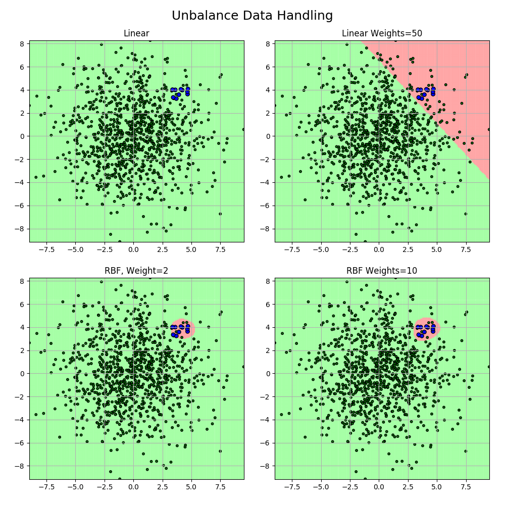
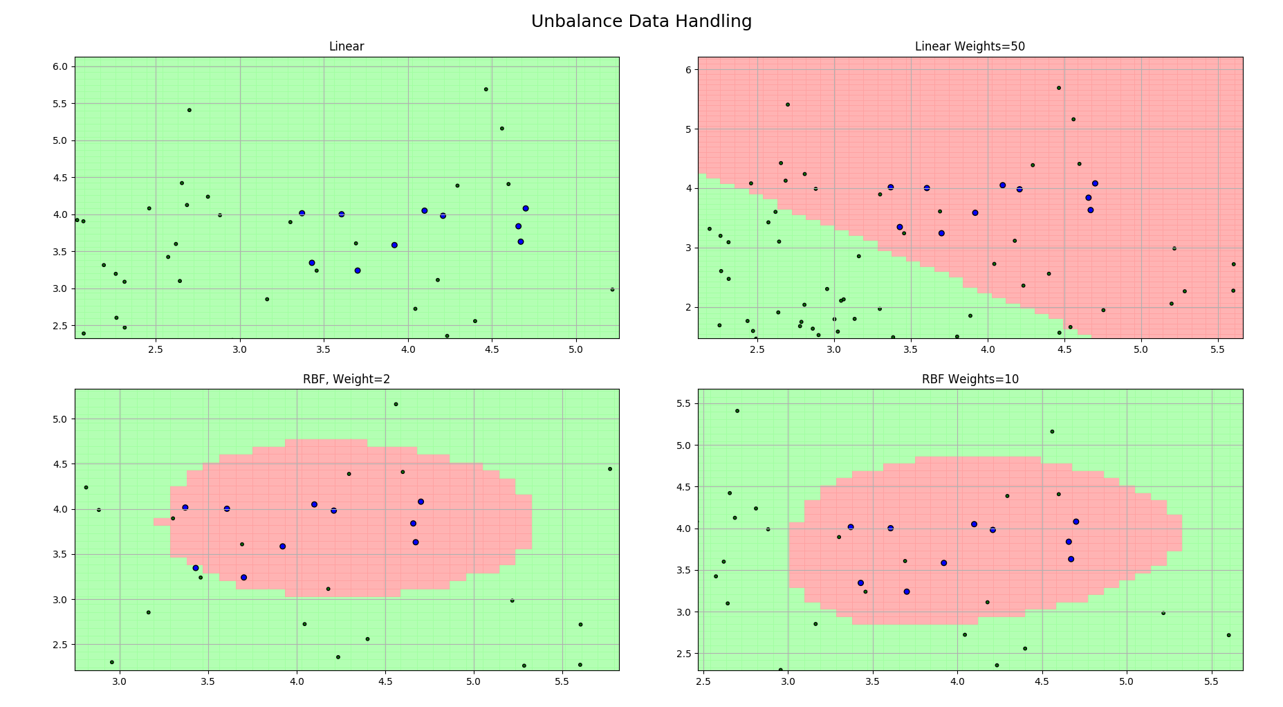
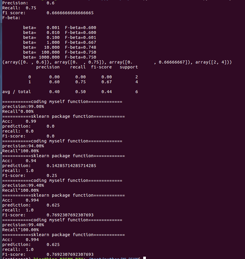
import numpy as np
from sklearn.metrics import accuracy_score
from sklearn.metrics import precision_score, recall_score, f1_score, fbeta_score
from sklearn.metrics import precision_recall_fscore_support, classification_report
from sklearn import svm
import matplotlib as mpl
import matplotlib.pyplot as plt
import warnings

def R_P():
	y_true = np.array([1, 1, 1, 1, 0, 0])
	y_hat = np.array([1, 0, 1, 1, 1, 1])

	print('Accuracy:\t', accuracy_score(y_true, y_hat))

	precision = precision_score(y_true, y_hat)
	print('Precision:\t', precision)

	recall = recall_score(y_true, y_hat)
	print('Recall:\t', recall)

	print('f1 score:\t', f1_score(y_true, y_hat))
	# print(2*(precision*recall)/(precision + recall))

	print('F-beta:\n')
	for beta in np.logspace(-3, 3, num=7, base=10):
		fbeta = fbeta_score(y_true, y_hat, beta=beta)
		print('\tbeta=%9.3f\tF-beta=%.3f' % (beta, fbeta))

	print(precision_recall_fscore_support(y_true, y_hat))
	print(classification_report(y_true, y_hat))

def show_accuracy(a, b):
	# 計算預測值和真實值一樣的正確率
	acc = a.ravel() == b.ravel()
	print('precision:%.2f%%' % ((100*float(acc.sum()))/a.size))

def show_recall(y, y_hat):
	# 提取出那個小樣本集中的預測和真實一樣的正確率
	print('Recall"%.2f%%' % (100*float(np.sum(y_hat[y == 1] == 1)) / np.extract(y == 1, y).size))


if __name__ == '__main__':
	# 忽視警告
	warnings.filterwarnings('ignore')
	# 保證每次生成的資料一樣
	np.random.seed(0)

	R_P()

	c1 = 990
	c2 = 10
	N = c1 + c2
	x_c1 = 3*np.random.randn(c1, 2)
	x_c2 = 0.5*np.random.randn(c2, 2) + (4, 4)
	x = np.vstack((x_c1, x_c2))
	y = np.ones(N)
	y[:c1] = -1
	# 顯示出大小
	s = np.ones(N) * 30
	s[:c1] = 10
	# 分類器
	clfs = [
		svm.SVC(C=1, kernel='linear'),
		svm.SVC(C=1, kernel='linear', class_weight={-1:1, 1:50}),
		svm.SVC(C=0.8, kernel='rbf', gamma=0.5, class_weight={-1:1, 1:2}),
		svm.SVC(C=0.8, kernel='rbf', gamma=0.5, class_weight={-1:1, 1:10}),
	]
	titles = 'Linear', 'Linear Weights=50', 'RBF, Weight=2', 'RBF Weights=10'

	x1_min, x1_max = x[:, 0].min(), x[:, 0].max()
	x2_min, x2_max = x[:, 1].min(), x[:, 1].max()
	# 生成網格取樣點
	x1, x2 = np.mgrid[x1_min:x1_max:200j, x2_min:x2_max:200j]
	# 測試點
	grid_test = np.stack((x1.flat, x2.flat), axis=1)
	cm_light = mpl.colors.ListedColormap(['#A0FFA0', '#FFA0A0'])
	cm_dark = mpl.colors.ListedColormap(['g', 'b'])

	plt.figure(figsize=(10, 10), facecolor='w')
	for i, clf in enumerate(clfs):
		clf.fit(x, y)
		y_hat = clf.predict(x)
		print('===========coding myself function=============')
		show_accuracy(y, y_hat)
		show_recall(y, y_hat)
		print('===========sklearn package function============')
		print('Acc:\t', accuracy_score(y, y_hat))
		print('prediction:\t', precision_score(y, y_hat, pos_label=1))
		print('recall:\t', recall_score(y, y_hat, pos_label=1))
		print('F1-score:\t', f1_score(y, y_hat, pos_label=1))

		# 開始畫圖
		plt.subplot(2, 2, i+1)
		grid_hat = clf.predict(grid_test)
		grid_hat.shape = x1.shape
		plt.pcolormesh(x1, x2, grid_hat, cmap=cm_light, alpha=0.8)
		plt.scatter(x[:, 0], x[:, 1], c=y, edgecolor='k', s=s, cmap=cm_dark)
		plt.xlim(x1_min, x1_max)
		plt.ylim(x2_min, x2_max)
		plt.title(titles[i])
		plt.grid()
	plt.suptitle('Unbalance Data Handling', fontsize=18)
	plt.tight_layout(2.0)
	plt.subplots_adjust(top=0.92)
	plt.show()