
Tensorflow實現LSTM識別MINIST
阿新 • • 發佈:2017-12-04
growth 輸入 應該 訓練 run 類別 out 運行 port
import tensorflow as tf
import numpy as np
from tensorflow.contrib import rnn
from tensorflow.examples.tutorials.mnist import input_data

config=tf.ConfigProto()
config.gpu_options.allow_growth=True
sess=tf.Session(config=config)

mnist = input_data.read_data_sets(‘MNIST_data‘,one_hot=True)
print(mnist.train.images.shape)
Extracting MNIST_data\train-images-idx3-ubyte.gz
Extracting MNIST_data\train-labels-idx1-ubyte.gz
Extracting MNIST_data\t10k-images-idx3-ubyte.gz
Extracting MNIST_data\t10k-labels-idx1-ubyte.gz
(55000, 784)
lr = 1e-3
input_size = 28 # 每個時刻的輸入特征是28維的,就是每個時刻輸入一行,一行有 28 個像素
timestep_size = 28 # 時序持續長度為28,即每做一次預測,需要先輸入28行 # 把784個點的字符信息還原成 28 * 28 的圖片
# 下面幾個步驟是實現 RNN / LSTM 的關鍵
####################################################################
# **RNN 的輸入shape = (batch_size, timestep_size, input_size)
X = tf.reshape(_X, [-1, 28, 28])
# 在 tf 1.2.1 版本中,可以通過下面方式來創建
def lstm_cell():
cell = rnn.LSTMCell(hidden_size, reuse=tf.get_variable_scope().reuse)
return rnn.DropoutWrapper(cell, output_keep_prob=keep_prob)
mlstm_cell = tf.contrib.rnn.MultiRNNCell([lstm_cell() for _ in range(layer_num)], state_is_tuple = True)
# **用全零來初始化state
init_state = mlstm_cell.zero_state(batch_size, dtype=tf.float32)
# **調用 dynamic_rnn() 來讓我們構建好的網絡運行起來
# ** 當 time_major==False 時, outputs.shape = [batch_size, timestep_size, hidden_size]
# ** 所以,可以取 h_state = outputs[:, -1, :] 作為最後輸出
# ** state.shape = [layer_num, 2, batch_size, hidden_size],
# ** 或者,可以取 h_state = state[-1][1] 作為最後輸出
# ** 最後輸出維度是 [batch_size, hidden_size]
outputs, state = tf.nn.dynamic_rnn(mlstm_cell, inputs=X, initial_state=init_state, time_major=False)
h_state = state[-1][1]W=tf.Variable(tf.truncated_normal([hidden_size,class_num],stddev=0.1),dtype=tf.float32)
bias=tf.Variable(tf.constant(0.1,shape=[class_num]),dtype=tf.float32)
y_pred=tf.nn.softmax(tf.matmul(h_state,W)+bias)
cross_entropy=-tf.reduce_mean(y*tf.log(y_pred))
train_op=tf.train.AdamOptimizer(lr).minimize(cross_entropy)
correct_prediction=tf.equal(tf.argmax(y_pred,1),tf.argmax(y,1))
accuracy=tf.reduce_mean(tf.cast(correct_prediction,"float"))
sess.run(tf.global_variables_initializer())
for i in range(2000):
_batch_size=128
batch=mnist.train.next_batch(_batch_size)
if (i+1)%200 ==0:
train_accuracy=sess.run(accuracy,feed_dict={
_X:batch[0],y:batch[1],keep_prob:1.0,batch_size:_batch_size
})
print(y_pred)
print(batch[0].shape)
print("Iter%d, step %d, training accuracy %g" % (mnist.train.epochs_completed,(i+1),train_accuracy))
sess.run(train_op,feed_dict={_X:batch[0],y:batch[1],keep_prob:0.5,batch_size:_batch_size})
print("test accuracy %g"% sess.run(accuracy,feed_dict={
_X:mnist.test.images,y:mnist.test.labels,keep_prob:1.0,batch_size:mnist.test.images.shape[0]
}))Tensor("Softmax_1:0", shape=(?, 10), dtype=float32)
(128, 784)
Iter5, step 200, training accuracy 0.9375
Tensor("Softmax_1:0", shape=(?, 10), dtype=float32)
(128, 784)
Iter5, step 400, training accuracy 0.976562
Tensor("Softmax_1:0", shape=(?, 10), dtype=float32)
(128, 784)
Iter6, step 600, training accuracy 0.96875
Tensor("Softmax_1:0", shape=(?, 10), dtype=float32)
(128, 784)
Iter6, step 800, training accuracy 0.984375
Tensor("Softmax_1:0", shape=(?, 10), dtype=float32)
(128, 784)
Iter6, step 1000, training accuracy 0.984375
Tensor("Softmax_1:0", shape=(?, 10), dtype=float32)
(128, 784)
Iter7, step 1200, training accuracy 0.984375
Tensor("Softmax_1:0", shape=(?, 10), dtype=float32)
(128, 784)
Iter7, step 1400, training accuracy 0.984375
Tensor("Softmax_1:0", shape=(?, 10), dtype=float32)
(128, 784)
Iter8, step 1600, training accuracy 0.992188
Tensor("Softmax_1:0", shape=(?, 10), dtype=float32)
(128, 784)
Iter8, step 1800, training accuracy 0.984375
Tensor("Softmax_1:0", shape=(?, 10), dtype=float32)
(128, 784)
Iter9, step 2000, training accuracy 0.992188
test accuracy 0.9863_batch_size=5
X_batch,y_batch=mnist.test.next_batch(_batch_size)
print(X_batch.shape,y_batch.shape)
_outputs,_state=sess.run([outputs,state],feed_dict={
_X:X_batch,y:y_batch,keep_prob:1.0,batch_size:_batch_size
})
print(‘outputs.shape=‘,np.asarray(_outputs).shape)
print(‘arr_state.shape=‘,np.asarray(_state).shape)
print(np.asarray(_state[-1][1]))
print(np.asarray(_state[0][1]))(5, 784) (5, 10)
outputs.shape= (5, 28, 256)
arr_state.shape= (2, 2, 5, 256)
[[-0.29114476 -0.84908068 -0.02608863 ..., -0.26059726 -0.41139302
0.59013247]
[-0.6596756 0.1405973 0.32068741 ..., 0.78834546 -0.85109633
-0.55030227]
[ 0.91946286 -0.6195702 0.00405734 ..., 0.50050467 0.4910633
-0.59666592]
[-0.89336431 0.21388607 0.50573528 ..., 0.75225669 0.6082601
-0.56074399]
[-0.36205587 -0.87424242 0.77999097 ..., 0.395004 -0.788903
-0.25867409]]
[[ 0.02811883 -0.1008996 0.03933555 ..., -0.26678833 -0.0076026
-0.04358114]
[-0.27545795 0.08285692 -0.09781252 ..., -0.40972584 0.14314541
0.83173752]
[-0.21126685 0.08805162 0.52263641 ..., -0.16019027 0.06584492
0.14457463]
[ 0.10716452 0.02429411 0.23363011 ..., 0.07705231 0.1158627
0.38137382]
[ 0.10278453 -0.19593915 0.18716493 ..., -0.15240444 -0.24707885
0.18361446]]import matplotlib.pyplot as pltprint(mnist.train.labels[4])[ 0. 0. 0. 0. 0. 0. 0. 1. 0. 0.]X3=mnist.train.images[3]
img3=X3.reshape([28,28])
print(img3.shape)
plt.imshow(img3,cmap=‘gray‘)
plt.show()(28, 28)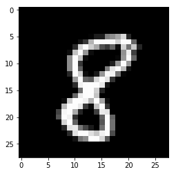
X3.shape=[-1,784]
y_batch=mnist.train.labels[0]
y_batch.shape=[-1,class_num]

X3_outputs=np.array(sess.run(outputs,feed_dict={
    _X:X3,y:y_batch,keep_prob:1.0,batch_size:1
}))
print(X3_outputs.shape)
X3_outputs.shape=[28,hidden_size]
print(X3_outputs.shape)
(1, 28, 256)
(28, 256)h_W=sess.run(W,feed_dict={
_X:X3,y:y_batch,keep_prob:1.0,batch_size:1
})
print(h_W)
h_bias=sess.run(bias,feed_dict={
_X:X3,y:y_batch,keep_prob:1.0,batch_size:1
})
print(h_bias)
bar_index=range(class_num)
for i in range(X3_outputs.shape[0]):
plt.subplot(7,4,i+1)
x3_h_shate=X3_outputs[i,:].reshape([-1,hidden_size])
pro=sess.run(tf.nn.softmax(tf.matmul(x3_h_shate,h_W)+h_bias))
plt.bar(bar_index,pro[0],width=0.2,align=‘center‘)
plt.axis(‘off‘)
plt.show()[[-0.08456483 0.08745969 -0.07621165 ..., -0.00773322 -0.15107249
0.10566489]
[ 0.26069802 0.13171725 0.0247799 ..., 0.08384562 0.06285298
0.03339371]
[-0.02133826 -0.08564553 0.09821648 ..., 0.05742728 0.02910433
0.17623523]
...,
[ 0.14126052 0.15447645 -0.08539373 ..., -0.27805188 0.12536794
0.0209918 ]
[-0.11653625 0.07422358 0.14709686 ..., -0.03686545 0.01324715
-0.12571484]
[-0.14584878 0.00623576 0.01669303 ..., 0.08890152 -0.1124042
-0.15828955]]
[ 0.0999197 0.14981271 0.07992077 0.08728788 0.08243027 0.11954871
0.08033348 0.12624525 0.10010903 0.08718728]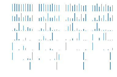
該文章主要參考An understandable example to implement Multi-LSTM for MNIST
在自己的github中也有內容Tensorflow_LSTM
並且發現如果多次使用jupyter調用 tf.contrib.rnn.MultiRNNCell那一段的內容容易導致程序報錯,後面的程序不能執行,具體原因不詳,若遇到問題,可restart and clear outputs 並且重新 start all即可
Tensorflow實現LSTM識別MINIST