
【 筆記 】定位演算法效能分析
目錄
PERFORMANCE ANALYSIS FOR LOCALIZATION ALGORITHMS
CRLB給出了使用相同資料的任何無偏估計可獲得的方差的下界,因此它可以作為與定位演算法的均方誤差(MSE)進行比較的重要基準。 然而,有偏估計的MSE可能小於CRLB。
在第1節中提供了在存在高斯噪聲的情況下使用TOA測量進行CRLB計算的過程。 在第2節中,我們給出了定位估計量的理論均值和MSE表示式,其推導基於成本函式的最小化或最大化。
1 CRLB Computation
生成CRLB的關鍵是構造相應的Fisher資訊矩陣(FIM)。 FIM逆的對角元素是可實現的最小方差值。 考慮公式2.1的一般測量模型,使用以下步驟總結計算CRLB的標準程式:


或者,當測量誤差為零 - 均值高斯分佈時,I(x)也可以計算為[20]
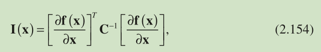
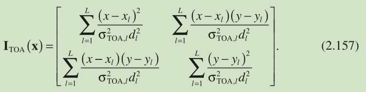
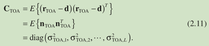
where C denotes the covariance matrix for n . We now utilize Equation 2.154 to determine the FIMs for positioning with TOA measure -ments based on Equations 2.8 and their associated noise covariance matrices, respectively. The FIM based on TOA measurements of Equation 2.5 , denoted by

注:


It is straightforward to show that

Employing Equations 2.156 and 2.11 , Equation 2.155 becomes
注:

2 Mean and Variance Analysis
When the position estimator corresponds to minimizing or maximizing a continuous cost function, the mean and MSE expressions of
當位置估計器對應於最小化或最大化連續成本函式時, 的均值和MSE表示式可以使用泰勒級數展開產生如下[25]。 設
是
的一般連續函式,估計
由其最小值或最大值給出。 這意味著

At small estimation error conditions, such that is located at a reasonable proximity of the ideal solution of x , using Taylor ’ s series to expand Equation 2.165 around x up to the first - order terms, we have
在小的估計誤差條件下,使得 位於x 的理想解的合理接近處,使用泰勒級數將公式2.165擴充套件到 x 到一階項,我們有

where and
are the corresponding Hessian matrix and gradient vector evaluated at the true location. When the second- order derivatives inside the Hessian matrix are smooth enough around x , we have [29] :
其中和
是在真實位置評估的相應Hessian矩陣和梯度向量。 當Hessian矩陣內的二階導數在 x 周圍足夠平滑時,我們有[29]:

Employing Equation 2.167 and taking the expected value of Equation 2.166 yield the mean of :
採用公式2.167並取公式2.166的預期值得出平均值:

When is an unbiased estimate of x ,
indicating that the last term in Equation 2.168 is a zero vector.
式子2.168的後半部分是零向量。由於Hessian的逆不為零,那麼梯度向量為零。
Utilizing Equations 2.166 and 2.167 again and the symmetric property of the Hessian matrix, we obtain the covariance for denoted by
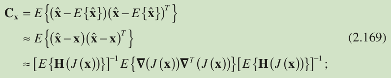
that is, the variances of the estimates of x and y are given by and
, respectively.
對角線上的數是x,y的方差。
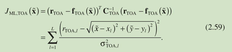
下面是具體的例項,以ML為例:
We first take the ML cost function for TOA-based positioning in Equation 2.59 , namely, , as an illustration. As
, the expected value of
can be easily determined with the use of Equations 2.61 – 2.64 as
注:


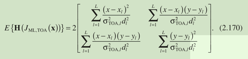
On the other hand, the expected value of is
![]()

注:

這意味著ML估計在其方差達到公式2.158中的CRLB的意義上是最優的。
均值和方差表示式也可以應用於線性方法,其對應於二次成本函式的最小化。 考慮公式2.119中的WLLS成本函式,相應的Hessian矩陣和梯度向量確定為


總體看來,挺困難的一些公式