
ML - 貸款使用者逾期情況分析1 - Baseline
文章目錄
任務
給定金融資料,預測貸款使用者是否會逾期。(status是標籤:0表示未逾期,1表示逾期。)
Task1 - 構建邏輯迴歸模型進行預測(在構建部分資料需要進行缺失值處理和資料型別轉換,如果不能處理,可以直接暴力刪除)
Task2 - 構建SVM和決策樹模型進行預測
Task3 - 構建xgboost和lightgbm模型進行預測
Task4 - 模型評估:記錄五個模型關於accuracy、precision,recall和f1-score、auc、roc的評分表格,畫出auc和roc曲線圖
總述
基本思路
主要分為以下幾個步驟:
1)資料集預覽
2)資料預處理:刪除無用特徵、字元型特徵編碼和缺失值填充。
3)特徵工程:略
4)模型選擇:LR、SVM(線性、多項式、高斯、sigmoid)、決策樹、XGB和lightGBM。
5)模型調參:略
6)模型評估:準確率、精準率和召回率、F1-score、AUC和ROC曲線。
7)最終結果
程式碼部分
1. 資料集預覽
import pandas as pd
data = pd.read_csv('data.csv')
print(data.shape)
data.head()
觀察輸出可知,資料集尺寸是(4754, 90)。
下面觀察一下各列的屬性名稱:
data.columns
輸出:‘low_volume_percent’,‘middle_volume_percent’,‘take_amount_in_later_12_month_highest’ …
2. 資料預處理
2.1 刪除無用特徵
# 'bank_card_no','source'的取值無區分度
# 'Unnamed: 0', 'custid', 'trade_no'和id_name'與預測無關
data.drop(['Unnamed: 0', 'custid', 'trade_no', 'bank_card_no', 'source', 'id_name'],
          axis=1, inplace=True)
日期特徵(暫時刪除, 以後再處理)
data.drop(['first_transaction_time', 'latest_query_time', 'loans_latest_time'],
          axis=1, inplace=True)
2.2 字元型特徵-編碼
data['reg_preference_for_trad'].value_counts()
輸出:
一線城市 3403
三線城市 1064
境外 150
二線城市 131
其他城市 4
對該特徵編碼如下:
dic = {}
for i, val in enumerate(list(data['reg_preference_for_trad'].unique())):
    dic[val] = i
data['reg_preference_for_trad'] = data['reg_preference_for_trad'].map(dic)
2.3 缺失特徵處理
觀察各列缺失值所佔比例,從輸出可以看出特徵student_feature 缺失值佔比超過一半,其餘特徵缺失值佔比較低。
for feature in data.columns:
    summ = data[feature].isnull().sum()
    if summ:
        print('%.4f'%(summ*100/4754), '%',  '--', feature)
1)student_feature 缺失佔比多, 需要用眾數填充;
data['student_feature'].value_counts()
輸出:
1.0 1754
2.0 2
用眾數1.0填充缺失值
data['student_feature'].fillna(1.0, inplace = True)
2)其餘特徵用均值填充。
for feature in data.columns:
    summ = data[feature].isnull().sum()
    if summ:
        data[feature].fillna(data[feature].mean(), inplace = True)
3. 特徵工程
略
4. 模型選擇
4.1 資料集劃分
features = [x for x in data.columns if x not in ['status']]
# 劃分訓練集測試集
from sklearn.model_selection import train_test_split
from sklearn.preprocessing import StandardScaler

X = data[features]
y = data.status

X_train, X_test, y_train, y_test = train_test_split(X, y, test_size=0.3,random_state=2333)

# 特徵歸一化
std = StandardScaler()
X_train = std.fit_transform(X_train)
X_test = std.transform(X_test)
4.2 LR模型
from sklearn.linear_model import LogisticRegression

lr = LogisticRegression()
lr.fit(X_train, y_train)
4.3 SVM模型
線性核函式、多項式核函式、高斯核函式、sigmoid核函式
新增probability=True,可使用predict_proba預測概率值。
from sklearn import svm

svm_linear = svm.SVC(kernel = 'linear', probability=True).fit(X_train, y_train)
svm_poly = svm.SVC(kernel = 'poly', probability=True).fit(X_train, y_train)
svm_rbf = svm.SVC(probability=True).fit(X_train, y_train)
svm_sigmoid = svm.SVC(kernel = 'sigmoid',probability=True).fit(X_train, y_train)
4.4 決策樹模型
樹模型,特徵不需歸一化。
from sklearn.tree import DecisionTreeClassifier

clf = DecisionTreeClassifier(max_depth=4)
clf.fit(X_train, y_train)
4.5 XGBoost模型
from xgboost.sklearn import XGBClassifier

xgb = XGBClassifier()
xgb.fit(X_train, y_train)
4.6 LightGBM模型
from lightgbm.sklearn import LGBMClassifier

lgb = LGBMClassifier()
lgb.fit(X_train, y_train)
5. 模型調參
略
6. 模型評估
觀察accuracy、precision,recall和f1-score、auc的取值,並畫出roc曲線圖
from sklearn.metrics import accuracy_score, precision_score, recall_score, f1_score
from sklearn.metrics import roc_auc_score,roc_curve, auc
import matplotlib.pyplot as plt
%matplotlib inline

def model_metrics(clf, X_train, X_test, y_train, y_test):
    # 預測
    y_train_pred = clf.predict(X_train)
    y_test_pred = clf.predict(X_test)

    y_train_proba = clf.predict_proba(X_train)[:,1]
    y_test_proba = clf.predict_proba(X_test)[:,1]

    # 準確率
    print('[準確率]', end = ' ')
    print('訓練集:', '%.4f'%accuracy_score(y_train, y_train_pred), end = ' ')
    print('測試集:', '%.4f'%accuracy_score(y_test, y_test_pred))

    # 精準率
    print('[精準率]', end = ' ')
    print('訓練集:', '%.4f'%precision_score(y_train, y_train_pred), end = ' ')
    print('測試集:', '%.4f'%precision_score(y_test, y_test_pred))

    # 召回率
    print('[召回率]', end = ' ')
    print('訓練集:', '%.4f'%recall_score(y_train, y_train_pred), end = ' ')
    print('測試集:', '%.4f'%recall_score(y_test, y_test_pred))

    # f1-score
    print('[f1-score]', end = ' ')
    print('訓練集:', '%.4f'%f1_score(y_train, y_train_pred), end = ' ')
    print('測試集:', '%.4f'%f1_score(y_test, y_test_pred))

    # auc取值:用roc_auc_score或auc
    print('[auc值]', end = ' ')
    print('訓練集:', '%.4f'%roc_auc_score(y_train, y_train_proba), end = ' ')
    print('測試集:', '%.4f'%roc_auc_score(y_test, y_test_proba))

    # roc曲線
    fpr_train, tpr_train, thresholds_train = roc_curve(y_train, y_train_proba, pos_label = 1)
    fpr_test, tpr_test, thresholds_test = roc_curve(y_test, y_test_proba, pos_label = 1)

    label = ["Train - AUC:{:.4f}".format(auc(fpr_train, tpr_train)),
             "Test - AUC:{:.4f}".format(auc(fpr_test, tpr_test))]
    plt.plot(fpr_train,tpr_train)
    plt.plot(fpr_test,tpr_test)
    plt.plot([0, 1], [0, 1], 'd--')
    plt.xlabel('False Positive Rate')
    plt.ylabel('True Positive Rate')
    plt.legend(label, loc = 4)
    plt.title("ROC curve")
# 邏輯迴歸
model_metrics(lr, X_train, X_test, y_train, y_test)
# 線性SVM
model_metrics(svm_linear, X_train, X_test, y_train, y_test)
# 多項式SVM
model_metrics(svm_poly, X_train, X_test, y_train, y_test)
# 高斯核SVM
model_metrics(svm_rbf, X_train, X_test, y_train, y_test)
# sigmoid-SVM
model_metrics(svm_sigmoid, X_train, X_test, y_train, y_test)
# 決策樹
model_metrics(dt, X_train, X_test, y_train, y_test)
# XGBoost
model_metrics(xgb, X_train, X_test, y_train, y_test)
# lightGBM
model_metrics(lgb, X_train, X_test, y_train, y_test)
7. 最終結果
| 模型 | 準確率 | 精準率 | 召回率 | F1-score | AUC值 | ROC曲線 |
|---|---|---|---|---|---|---|
| 邏輯迴歸 | 訓練集:0.7995 測試集: 0.8024 | 訓練集: 0.7094 測試集: 0.7052 | 訓練集: 0.3488 測試集: 0.3456 | 訓練集: 0.4677 測試集: 0.4639 | 訓練集: 0.8054 測試集: 0.8050 | 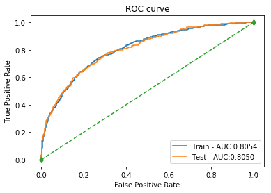 |
| SVM_linear | 訓練集: 0.7908 測試集: 0.7947 | 訓練集: 0.7647 測試集: 0.7885 | 訓練集: 0.2476 測試集: 0.2323 | 訓練集: 0.3741 測試集: 0.3589 | 訓練集: 0.8042 測試集: 0.8092 | 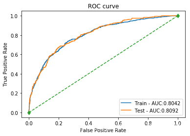 |
| SVM_poly | 訓練集: 0.8284 測試集: 0.7554 | 訓練集: 0.9786 測試集: 0.5208 | 訓練集: 0.3274 測試集: 0.1416 | 訓練集: 0.4906 測試集: 0.2227 | 訓練集: 0.9391 測試集: 0.7117 | 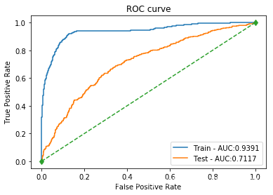 |
| SVM_rbf | 訓練集: 0.8266 測試集: 0.7975 | 訓練集: 0.9046 測試集: 0.7963 | 訓練集: 0.3500 測試集: 0.2436 | 訓練集: 0.5047 測試集: 0.3731 | 訓練集: 0.9170 測試集: 0.7680 | 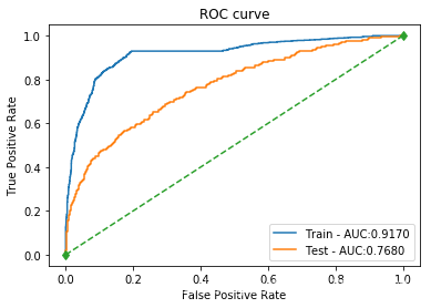 |
| SVM_sigmoid | 訓練集: 0.7205 測試集: 0.7379 | 訓練集: 0.4373 測試集: 0.4662 | 訓練集: 0.3738 測試集: 0.4108 | 訓練集: 0.4031 測試集: 0.4367 | 訓練集: 0.6600 測試集: 0.6784 | 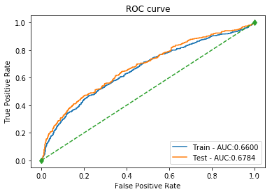 |
| 決策樹 | 訓練集: 0.7920 測試集: 0.7737 | 訓練集: 0.6581 測試集: 0.5862 | 訓練集: 0.3667 測試集: 0.2890 | 訓練集: 0.4709 測試集: 0.3871 | 訓練集: 0.7727 測試集: 0.7468 | 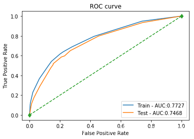 |
| XGBoost | 訓練集: 0.8521 測試集: 0.8045 | 訓練集: 0.8718 測試集: 0.7079 | 訓練集: 0.4857 測試集: 0.3569 | 訓練集: 0.6239 測試集: 0.4746 | 訓練集: 0.9166 測試集: 0.7972 | 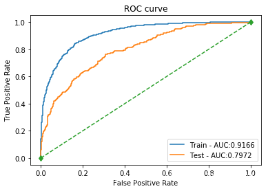 |
| LightGBM | 訓練集: 0.9949 測試集: 0.7961 | 訓練集: 1.0000 測試集: 0.6550 | 訓練集: 0.9798 測試集: 0.3711 | 訓練集: 0.9898 測試集: 0.4738 | 訓練集: 1.0000 測試集: 0.7869 |  |
遇到的問題
1)pd.read_csv讀取檔案時,utf-8的編碼問題。
解決方法:reference1
2)裝完xgboost後在notebook總是顯示如下錯誤:ImportError: cannot import name ‘MultiIndex’。
解決方法:更新scipy和xgboost後還是沒有解決;後來重啟了一下jupyter就好了…
3)畫ROC曲線時, tpr取值為nan
解決方法:注意roc_curve裡的幾個引數:第二項為真實y與預測的scores而不是y_pred,而pos_label=1指在y中標籤為1的是標準陽性標籤,其餘值是陰性。
4)SVM用函式clf.predict_proba()時候報錯如下:
AttributeError: predict_proba is not available when probability=False
解決方法:clf = SVC()預設情況probability=False,新增probability=True
Reference
1)python問題–UnicodeDecodeError: ‘utf-8’ codec can’t decode byte 0xff in position 0: invalid start byte
2)ML實操 - 貸款使用者逾期情況分析
More
程式碼參見Github: https://github.com/libihan/Exercise-ML