
通過一文入門Matplotlib
阿新 • • 發佈:2018-12-06
1、開始
import matplotlib.pyplot as plt
import numpy as np

x = np.linspace(-1,1,50)#從(-1,1)均勻取50個點
y = 2 * x

plt.plot(x,y)
plt.show()
2、Figure物件
import matplotlib.pyplot as plt
import numpy as np

x = np.linspace(-1,1,50)
y1 = x ** 2
y2 = x * 2
#這個是第一個figure物件,下面的內容都會在第一個figure中顯示
plt.figure()
plt.plot(x,y1)
#這裡第二個figure物件
plt.figure(num = 3,figsize = (10,5))
plt.plot(x,y2)
plt.show()

- 我們看上面的每個影象的視窗,可以看出figure並沒有從1開始然後到2,這是因為我們在建立第二個figure物件的時候,指定了一個num = 3的引數,所以第二個視窗標題上顯示的figure3。
- 對於每一個視窗,我們也可以對他們分別去指定視窗的大小。也就是figsize引數。
- 若我們想讓他們的線有所區別,我們可以用下面語句進行修改。
plt.plot(x,y2,color = 'red',linewidth = 3.0,linestyle = '--')
3、設定座標軸
import matplotlib.pyplot as plt
import numpy as np

x = np.linspace(-1,1,50)
y = x *2

plt.plot(x,y)
plt.show()
預設的橫座標:

#在plt.show()之前新增
plt.xlim((0,2))
plt.ylim((-2,2))

給橫縱座標設定名稱:
import matplotlib.pyplot as plt
import numpy as np

x = np.linspace(-1,1,50)
y = x * 2

plt.xlabel("x'slabel")#x軸上的名字
plt.ylabel("y's;abel")#y軸上的名字
plt.plot(x,y,color='green',linewidth = 3)
plt.show()

把座標軸換成不同的單位:
new_ticks = np.linspace(-1,2,5)
plt.xticks(new_ticks)
#在對應座標處更換名稱
plt.yticks([-2,-1,0,1,2],['really bad','b','c','d','good'])

那麼如果我想把座標軸上的字型更改成數學的那種形式:
#在對應座標處更換名稱
plt.yticks([-2,-1,0,1,2],[r'$really\ bad$',r'$b$',r'$c\ \alpha$','d','good'])

注意:
- 我們如果要使用空格的話需要進行對空格的轉義"\ "這種轉義才能輸出空格;
- 我們可以在裡面加一些數學的公式,如"\alpha"來表示 。
如何去更換座標原點,座標軸呢?我們在plt.show()之前:
#gca = 'get current axis'
#獲取當前的這四個軸
ax = plt.gca()
#設定脊樑(也就是包圍在圖示四周的預設黑線)
#所以設定脊樑的時候,一共有四個方位
ax.spines['right'].set_color('r')
ax.spines['top'].set_color('none')

#將底部脊樑作為x軸
ax.xaxis.set_ticks_position('bottom')
#ACCEPTS:['top' | 'bottom' | 'both'|'default'|'none']

#設定x軸的位置(設定底的時候依據的是y軸)
ax.spines['bottom'].set_position(('data',0))
#the 1st is in 'outward' |'axes' | 'data'
#axes : precentage of y axis
#data : depend on y data

ax.yaxis.set_ticks_position('left')
# #ACCEPTS:['top' | 'bottom' | 'both'|'default'|'none']

#設定左脊樑(y軸)依據的是x軸的0位置
ax.spines['left'].set_position(('data',0))

4.legend圖例
我們很多時候會再一個figures中去新增多條線,那我們如何去區分多條線呢?這裡就用到了legend。
#簡單的使用
l1, = plt.plot(x, y1, label='linear line')
l2, = plt.plot(x, y2, color='red', linewidth=1.0, linestyle='--', label='square line')

#簡單的設定legend(設定位置)
#位置在右上角
plt.legend(loc = 'upper right')

l1, = plt.plot(x, y1, label='linear line')
l2, = plt.plot(x, y2, color='red', linewidth=1.0, linestyle='--', label='square line')


plt.legend(handles = [l1,l2],labels = ['up','down'],loc = 'best')
#the ',' is very important in here l1, = plt...and l2, = plt...for this step
"""legend( handles=(line1, line2, line3),
           labels=('label1', 'label2', 'label3'),
           'upper right')
    shadow = True 設定圖例是否有陰影
    The *loc* location codes are::
          'best' : 0,
          'upper right'  : 1,
          'upper left'   : 2,
          'lower left'   : 3,
          'lower right'  : 4,
          'right'        : 5,
          'center left'  : 6,
          'center right' : 7,
          'lower center' : 8,
          'upper center' : 9,
          'center'       : 10,"""

這裡需要注意的是:
- 如果我們沒有在legend方法的引數中設定labels,那麼就會使用畫線的時候,也就是plot方法中的指定的label引數所指定的名稱,當然如果都沒有的話就會丟擲異常;
- 其實我們plt.plot的時候返回的是一個線的物件,如果我們想在handle中使用這個物件,就必須在返回的名字的後面加一個","號;
legend = plt.legend(handles = [l1,l2],labels = ['hu','tang'],loc = 'upper center',shadow = True)
frame = legend.get_frame()
frame.set_facecolor('r')#或者0.9...

5.在圖片上加一些標註annotation
在圖片上加註解有兩種方式:
import matplotlib.pyplot as plt
import numpy as np

x = np.linspace(-3,3,50)
y = 2*x + 1

plt.figure(num = 1,figsize =(8,5))
plt.plot(x,y)

ax = plt.gca()
ax.spines['right'].set_color('none')
ax.spines['top'].set_color('none')

#將底下的作為x軸
ax.xaxis.set_ticks_position('bottom')
#並且data,以y軸的資料為基本
ax.spines['bottom'].set_position(('data',0))

#將左邊的作為y軸
ax.yaxis.set_ticks_position('left')
ax.spines['left'].set_position(('data',0))

print("-----方式一-----")
x0 = 1
y0 = 2*x0 + 1
plt.plot([x0,x0],[0,y0],'k--',linewidth = 2.5)
plt.scatter([x0],[y0],s = 50,color='b')
plt.annotate(r'$2x+1 = %s$'% y0,xy = (x0,y0),xycoords = 'data',
             xytext=(+30,-30),textcoords = 'offset points',fontsize = 16
             ,arrowprops = dict(arrowstyle='->',
                                connectionstyle="arc3,rad=.2"))
plt.show()

plt.annotate(r'$2x+1 = %s$'% y0,xy = (x0,y0),xycoords = 'data',
             xytext=(+30,-30),textcoords = 'offset points',fontsize = 16
             ,arrowprops = dict(arrowstyle='->',
                                connectionstyle="arc3,rad=.2"))
注意:
- xy就是需要進行註釋的點的橫縱座標;
- xycoords = 'data'說明的是要註釋點的xy的座標是以橫縱座標軸為基準的;
- xytext=(+30,-30)和textcoords='data'說明了這裡的文字是基於標註的點的x座標的偏移+30以及標註點y座標-30位置,就是我們要進行註釋文字的位置;
- fontsize = 16就說明字型的大小;
- arrowprops = dict()這個是對於這個箭頭的描述,arrowstyle='->'這個是箭頭的型別,connectionstyle="arc3,rad=.2"這兩個是描述我們的箭頭的弧度以及角度的。
print("-----方式二-----")
plt.text(-3.7,3,r'$this\ is\ the\ some\ text. \mu\ \sigma_i\ \alpha_t$',
         fontdict={'size':16,'color':'r'})

這裡先介紹一下plot中的一個引數:
import matplotlib.pyplot as plt
import numpy as np

x = np.linspace(-3,3,50)
y1 = 0.1*x
y2 = x**2

plt.figure()
#zorder控制繪圖順序
plt.plot(x,y1,linewidth = 10,zorder = 2,label = r'$y_1\ =\ 0.1*x$')
plt.plot(x,y2,linewidth = 10,zorder = 1,label = r'$y_2\ =\ x^{2}$')

plt.legend(loc = 'lower right')

plt.show()

如果改成:
#zorder控制繪圖順序
plt.plot(x,y1,linewidth = 10,zorder = 1,label = r'$y_1\ =\ 0.1*x$')
plt.plot(x,y2,linewidth = 10,zorder = 2,label = r'$y_2\ =\ x^{2}$')

下面我們看一下這個圖:
import matplotlib.pyplot as plt
import numpy as np

x = np.linspace(-3,3,50)
y1 = 0.1*x
y2 = x**2

plt.figure()
#zorder控制繪圖順序
plt.plot(x,y1,linewidth = 10,zorder = 1,label = r'$y_1\ =\ 0.1*x$')
plt.plot(x,y2,linewidth = 10,zorder = 2,label = r'$y_2\ =\ x^{2}$')

plt.ylim(-2,2)

ax = plt.gca()
ax.spines['right'].set_color('none')
ax.spines['top'].set_color('none')

ax.xaxis.set_ticks_position('bottom')
ax.spines['bottom'].set_position(('data',0))
ax.yaxis.set_ticks_position('left')
ax.spines['left'].set_position(('data',0))

plt.show()

從上面看,我們可以看見我們軸上的座標被掩蓋住了,那麼我們怎麼去修改他呢?
print(ax.get_xticklabels())
print(ax.get_yticklabels())

for label in ax.get_xticklabels() + ax.get_yticklabels():
    label.set_fontsize(12)
    label.set_bbox(dict(facecolor = 'white',edgecolor='none',alpha = 0.8,zorder = 2))

<a list of 9 Text xticklabel objects>
<a list of 9 Text yticklabel objects>

這裡需要注意:
- ax.get_xticklabels()獲取得到就是座標軸上的數字;
- set_bbox()這個bbox就是那座標軸上的數字的那一小塊區域,從結果我們可以很明顯的看出來;
- facecolor = 'white',edgecolor='none,第一個引數表示的這個box的前面的背景,邊上的顏色。
6.畫圖的種類
1.scatter散點圖
import matplotlib.pyplot as plt
import numpy as np

n = 1024
X = np.random.normal(0,1,n)
Y = np.random.normal(0,1,n)
T = np.arctan2(Y,X)#for color later on

plt.scatter(X,Y,s = 75,c = T,alpha = .5)

plt.xlim((-1.5,1.5))
plt.xticks([])#ignore xticks
plt.ylim((-1.5,1.5))
plt.yticks([])#ignore yticks
plt.show()

2.柱狀圖
import matplotlib.pyplot as plt
import numpy as np

n = 12
X = np.arange(n)
Y1 = (1 - X/float(n)) * np.random.uniform(0.5,1.0,n)
Y2 = (1 - X/float(n)) * np.random.uniform(0.5,1.0,n)
#facecolor:表面的顏色;edgecolor:邊框的顏色
plt.bar(X,+Y1,facecolor = '#9999ff',edgecolor = 'white')
plt.bar(X,-Y2,facecolor = '#ff9999',edgecolor = 'white')
#描繪text在圖表上
# plt.text(0 + 0.4, 0 + 0.05,"huhu")
for x,y in zip(X,Y1):
    #ha : horizontal alignment
    #va : vertical alignment
    plt.text(x + 0.01,y+0.05,'%.2f'%y,ha = 'center',va='bottom')

for x,y in zip(X,Y2):
    # ha : horizontal alignment
    # va : vertical alignment
    plt.text(x+0.01,-y-0.05,'%.2f'%(-y),ha='center',va='top')

plt.xlim(-.5,n)
plt.yticks([])
plt.ylim(-1.25,1.25)
plt.yticks([])
plt.show()

3.Contours等高線圖
import matplotlib.pyplot as plt
import numpy as np

def f(x,y):
    #the height function
    return (1-x/2 + x**5+y**3) * np.exp(-x **2 -y**2)

n = 256
x = np.linspace(-3,3,n)
y = np.linspace(-3,3,n)
#meshgrid函式用兩個座標軸上的點在平面上畫網格。
X,Y = np.meshgrid(x,y)

#use plt.contourf to filling contours
#X Y and value for (X,Y) point
#這裡的8就是說明等高線分成多少個部分,如果是0則分成2半
#則8是分成10半
#cmap找對應的顏色,如果高=0就找0對應的顏色值,
plt.contourf(X,Y,f(X,Y),8,alpha = .75,cmap = plt.cm.hot)

#use plt.contour to add contour lines
C = plt.contour(X,Y,f(X,Y),8,colors = 'black',linewidth = .5)

#adding label
plt.clabel(C,inline = True,fontsize = 10)

#ignore ticks
plt.xticks([])
plt.yticks([])

plt.show()

4.image圖片
import matplotlib.pyplot as plt
import numpy as np

#image data
a = np.array([0.313660827978, 0.365348418405, 0.423733120134,
              0.365348418405, 0.439599930621, 0.525083754405,
              0.423733120134, 0.525083754405, 0.651536351379]).reshape(3,3)

'''
for the value of "interpolation",check this:
http://matplotlib.org/examples/images_contours_and_fields/interpolation_methods.html
for the value of "origin"= ['upper', 'lower'], check this:
http://matplotlib.org/examples/pylab_examples/image_origin.html
'''
#顯示影象
#這裡的cmap='bone'等價於plt.cm.bone
plt.imshow(a,interpolation = 'nearest',cmap = 'bone' ,origin = 'up')
#顯示右邊的欄
plt.colorbar(shrink = .92)

#ignore ticks
plt.xticks([])
plt.yticks([])

plt.show()

5.3D資料
import numpy as np
import matplotlib.pyplot as plt
from mpl_toolkits.mplot3d import Axes3D

fig = plt.figure()
ax = Axes3D(fig)
#X Y value
X = np.arange(-4,4,0.25)
Y = np.arange(-4,4,0.25)
X,Y = np.meshgrid(X,Y)
R = np.sqrt(X**2 + Y**2)
#hight value
Z = np.sin(R)

ax.plot_surface(X, Y, Z, rstride=1, cstride=1, cmap=plt.get_cmap('rainbow'))
"""
============= ================================================
        Argument      Description
        ============= ================================================
        *X*, *Y*, *Z* Data values as 2D arrays
        *rstride*     Array row stride (step size), defaults to 10
        *cstride*     Array column stride (step size), defaults to 10
        *color*       Color of the surface patches
        *cmap*        A colormap for the surface patches.
        *facecolors*  Face colors for the individual patches
        *norm*        An instance of Normalize to map values to colors
        *vmin*        Minimum value to map
        *vmax*        Maximum value to map
        *shade*       Whether to shade the facecolors
        ============= ================================================
"""

# I think this is different from plt12_contours
ax.contourf(X, Y, Z, zdir='z', offset=-2, cmap=plt.get_cmap('rainbow'))
"""
==========  ================================================
        Argument    Description
        ==========  ================================================
        *X*, *Y*,   Data values as numpy.arrays
        *Z*
        *zdir*      The direction to use: x, y or z (default)
        *offset*    If specified plot a projection of the filled contour
                    on this position in plane normal to zdir
        ==========  ================================================
"""
ax.set_zlim(-2, 2)
plt.show()

7.多圖合併展示
1.使用subplot函式
import matplotlib.pyplot as plt

plt.figure(figsize = (6,5))

ax1 = plt.subplot(3,1,1)
ax1.set_title("ax1 title")
plt.plot([0,1],[0,1])

#這種情況下如果再數的話以334為標準了,
#把上面的第一行看成是3個列
ax2 = plt.subplot(334)
ax2.set_title("ax2 title")

ax3 = plt.subplot(335)
ax4 = plt.subplot(336)
ax5 = plt.subplot(325)
ax6 = plt.subplot(326)

plt.show()

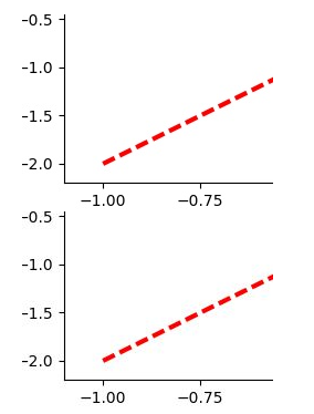
import matplotlib.pyplot as plt

plt.figure(figsize = (6,4))
#plt.subplot(n_rows,n_cols,plot_num)
plt.subplot(211)
# figure splits into 2 rows, 1 col, plot to the 1st sub-fig
plt.plot([0, 1], [0, 1])

plt.subplot(234)
# figure splits into 2 rows, 3 col, plot to the 4th sub-fig
plt.plot([0, 1], [0, 2])

plt.subplot(235)
# figure splits into 2 rows, 3 col, plot to the 5th sub-fig
plt.plot([0, 1], [0, 3])

plt.subplot(236)
# figure splits into 2 rows, 3 col, plot to the 6th sub-fig
plt.plot([0, 1], [0, 4])

plt.tight_layout()
plt.show()

2.分格顯示
#method 1: subplot2grid
import matplotlib.pyplot as plt
plt.figure()
#第一個引數shape也就是我們網格的形狀
#第二個引數loc,位置,這裡需要注意位置是從0開始索引的
#第三個引數colspan跨多少列,預設是1
#第四個引數rowspan跨多少行,預設是1
ax1 = plt.subplot2grid((3,3),(0,0),colspan = 3,rowspan = 1)
#如果為他設定一些屬性的話,如plt.title,則用ax1的話
#ax1.set_title(),同理可設定其他屬性
ax1.set_title("ax1_title")

ax2 = plt.subplot2grid((3,3),(1,0),colspan = 2,rowspan = 1)
ax3 = plt.subplot2grid((3,3),(1,2),colspan = 1,rowspan = 2)
ax4 = plt.subplot2grid((3,3),(2,0),colspan = 1,rowspan = 1)
ax5 = plt.subplot2grid((3,3),(2,1),colspan = 1,rowspan = 1)

plt.show()

#method 2:gridspec
import matplotlib.pyplot as plt
import matplotlib.gridspec as gridspec

plt.figure()
gs = gridspec.GridSpec(3,3)
#use index from 0
ax1 = plt.subplot(gs[0,:])
ax1.set_title("ax1 title")

ax2 = plt.subplot(gs[1,:2])
ax2.plot([1,2],[3,4],'r')

ax3 = plt.subplot(gs[1:,2:])
ax4 = plt.subplot(gs[-1,0])
ax5 = plt.subplot(gs[-1,-2])

plt.show()

#method 3 :easy to define structure
#這種方式不能生成指定跨行列的那種
import matplotlib.pyplot as plt
#(ax11,ax12),(ax13,ax14)代表了兩行
#f就是figure物件,
#sharex:是否共享x軸
#sharey:是否共享y軸
f,((ax11,ax12),(ax13,ax14)) = plt.subplots(2,2,sharex = True,sharey = True)
ax11.set_title("a11 title")
ax12.scatter([1,2],[1,2])

plt.show()

3.圖中圖
import matplotlib.pyplot as plt

fig = plt.figure()
x = [1,2,3,4,5,6,7]
y = [1,3,4,2,5,8,6]

#below are all percentage
left, bottom, width, height = 0.1, 0.1, 0.8, 0.8
#使用plt.figure()顯示的是一個空的figure
#如果使用fig.add_axes會新增軸
ax1 = fig.add_axes([left, bottom, width, height])# main axes
ax1.plot(x,y,'r')
ax1.set_xlabel('x')
ax1.set_ylabel('y')
ax1.set_title('title')

ax2 = fig.add_axes([0.2, 0.6, 0.25, 0.25])  # inside axes
ax2.plot(y, x, 'b')
ax2.set_xlabel('x')
ax2.set_ylabel('y')
ax2.set_title('title inside 1')

# different method to add axes
####################################
plt.axes([0.6, 0.2, 0.25, 0.25])
plt.plot(y[::-1], x, 'g')
plt.xlabel('x')
plt.ylabel('y')
plt.title('title inside 2')

plt.show()

4.次座標軸
# 使用twinx是新增y軸的座標軸
# 使用twiny是新增x軸的座標軸
import matplotlib.pyplot as plt
import numpy as np

x = np.arange(0,10,0.1)
y1 = 0.05 * x ** 2
y2 = -1 * y1

fig,ax1 = plt.subplots()

ax2 = ax1.twinx()
ax1.plot(x,y1,'g-')
ax2.plot(x,y2,'b-')

ax1.set_xlabel('X data')
ax1.set_ylabel('Y1 data',color = 'g')
ax2.set_ylabel('Y2 data',color = 'b')

plt.show()

8.animation動畫
import numpy as np
from matplotlib import pyplot as plt
from matplotlib import animation

fig,ax = plt.subplots()

x = np.arange(0,2*np.pi,0.01)
#因為這裡返回的是一個列表,但是我們只想要第一個值
#所以這裡需要加,號
line, = ax.plot(x,np.sin(x))

def animate(i):
    line.set_ydata(np.sin(x + i/10.0))#updata the data
    return line,

def init():
    line.set_ydata(np.sin(x))
    return line,


# call the animator.  blit=True means only re-draw the parts that have changed.
# blit=True dose not work on Mac, set blit=False
# interval= update frequency
#frames幀數
ani = animation.FuncAnimation(fig=fig, func=animate, frames=100, init_func=init,
                              interval=20, blit=False)

plt.show()
以上內容均學習自莫煩教程。