本文受到樊哲勇老師部落格中的一個用matlab實現的50行的遺傳演算法程式 啟發，並在此基礎上增加了註釋，並將遺傳演算法中的一些關鍵步驟重寫了函式，使得整個程式碼結構、邏輯清晰。程式碼主要有六個檔案：

main.m : 主函式，在這裡呼叫遺傳演算法

my_ga.m : 完整的遺傳演算法函式

my_gene.m : 基因編碼，產生初代基因

my_fitness.m : 適應度函式

my_cross.m : 用於染色體交叉

my_mutations.m : 基於基因突變突變方式

下面我將解釋每個檔案：

main.m 主函式

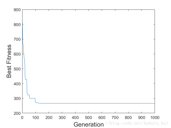
clear; close all;



% 呼叫 my_ga 進行計算

[best_fitness, elite, generation] = my_ga(15, 'my_fitness', 100, 50, 0.3, 1000, 1.0e-6);

%    number_of_variables, ...    % 求解問題的引數個數
%    fitness_function, ...       % 自定義適應度函式名
%    population_size, ...        % 種群規模（每一代個體數目）
%    parent_number, ...          % 每一代中保持不變的數目（除了變異）
%    mutation_rate, ...          % 變異概率
%    maximal_generation, ...     % 最大演化代數
%    minimal_cost ...            % 最小目標值（函式值越小，則適應度越高）

min(best_fitness)      % 最短路徑
elite(generation,:)	   % 最優路徑

% 最佳適應度的演化情況
figure
plot(best_fitness);
xlabel('Generation','fontsize',15);
ylabel('Best Fitness','fontsize',15);
 

在主函式中主要呼叫遺傳演算法函式，傳入的引數主要有引數個數、自定義適應度函式名稱、種群規模、種群中父代的個數、變異概率、最大演化代數和最小目標值。

my_ga.m 遺傳演算法函式

function [best_fitness, elite, generation, last_generation] = my_ga( ...
    number_of_variables, ...    % 求解問題的引數個數
    fitness_function, ...       % 自定義適應度函式名
    population_size, ...        % 種群規模（每一代個體數目）
    parent_number, ...          % 每一代中保持不變的數目（除了變異）
    mutation_rate, ...          % 變異概率
    maximal_generation, ...     % 最大演化代數
    minimal_cost ...            % 最小目標值（函式值越小，則適應度越高）
)

% 累加概率
% 假設 parent_number = 10
% 分子 parent_number:-1:1 用於生成一個數列
% 分母 sum(parent_number:-1:1) 是一個求和結果（一個數）
%
% 分子 10     9     8     7     6     5     4     3     2     1
% 分母 55
% 相除 0.1818    0.1636    0.1455    0.1273    0.1091    0.0909    0.0727    0.0545    0.0364    0.0182
% 累加 0.1818    0.3455    0.4909    0.6182    0.7273    0.8182    0.8909    0.9455    0.9818    1.0000
%
% 運算結果可以看出, 累加概率函式是一個從0到1增長得越來越慢的函式
% 因為後面加的概率越來越小（數列是降虛排列的）
cumulative_probabilities = cumsum((parent_number:-1:1) / sum(parent_number:-1:1)); % 1個長度為parent_number的數列,其值為[0,1]，越往後越慢

% 最佳適應度
% 每一代的最佳適應度都先初始化為1
best_fitness = ones(maximal_generation, 1);

% 精英
% 每一代的精英的引數值都先初始化為0
elite = zeros(maximal_generation, number_of_variables);

% 子女數量
% 種群數量 - 父母數量（父母即每一代中不發生改變的個體）
child_number = population_size - parent_number; % 每一代子女的數目

% 初始化種群 --- 產生基因
% population_size 對應矩陣的行，每一行表示1個個體，行數=個體數（種群數量）
% number_of_variables 對應矩陣的列，列數=引數個數（個體特徵由這些引數表示） 
% population = rand(population_size, number_of_variables);
population = my_gene(population_size, number_of_variables);

last_generation = 0; % 記錄跳出迴圈時的代數

% 後面的程式碼都在for迴圈中
for generation = 1 : maximal_generation % 演化迴圈開始
    
    % feval把資料帶入到一個定義好的函式控制代碼中計算
    % 把population矩陣帶入fitness_function函式計算
    cost = feval(fitness_function, population); % 計算所有個體的適應度（population_size*1的矩陣）

    % index記錄排序後每個值原來的行數
    [cost, index] = sort(cost); % 將適應度函式值從小到大排序

    % index(1:parent_number) 
    % 前parent_number個cost較小的個體在種群population中的行數
    % 選出這部分(parent_number個)個體作為父母，其實parent_number對應交叉概率
    population = population(index(1:parent_number), :); % 先保留一部分較優的個體
    % 可以看出population矩陣是不斷變化的

    % cost在經過前面的sort排序後，矩陣已經改變為升序的
    % cost(1)即為本代的最佳適應度
    best_fitness(generation) = cost(1); % 記錄本代的最佳適應度

    % population矩陣第一行為本代的精英個體
    elite(generation, :) = population(1, :); % 記錄本代的最優解（精英）

    % 若本代的最優解已足夠好，則停止演化
    if best_fitness(generation) < minimal_cost; 
        last_generation = generation;
        break; 
    end
    % 交叉變異產生新的種群
        
    % 染色體交叉開始
    population = my_cross(population, cumulative_probabilities, child_number, number_of_variables, parent_number);
    % 染色體交叉結束
     
    % 染色體變異開始
    mutation_population = population(2:population_size, :); % 精英不參與變異，所以從2開始
    population(2:population_size, :) = my_mutations(mutation_population, mutation_rate); % 發生變異之後的種群
    % 染色體變異結束
     
    if(mod(generation, 100) == 0)
        disp(['程式已迭代：', num2str(generation) ,'次']);
    end
   
end % 演化迴圈結束
 

我直接跳過前面的部分引數的初始化的過程，直接說一些關鍵的點。

在進入迴圈之前，先呼叫my_gene函式生成初代種群，然後進入迴圈中。在每次迴圈中，先進行適應度計算，這個時候呼叫的是函式my_fitness，將計算好的適應度函式值從小到大進行排序，保留前parent_number個體作為父代，後面的個體就淘汰了，並記錄本代中最優的適應度和路徑(即為第一個資料)。因為淘汰了部分個體，所以要從保留下來的父代中生成子代，並組成下一次迭代的種群，這個時候就呼叫了函式my_cross，主要通過染色體的交叉來實現，這樣一個兩個父代就可以產生兩個子代。為了避免演算法陷入區域性最優解，要使部分染色體進行變異，變異呼叫的函式就my_mutations

下面我將按照上一段所提到的函式順序，依次來介紹這些函式：

my_gene.m 產生初代種群

function population = my_gene(population_size, number_of_variables)
  % 產生初代基因（基因編碼）
  % population_size ： 種群規模
  % number_of_variables ： 變數的個數/基因的長度
  % population = rand(population_size, number_of_variables);
  
  population = rand(population_size, number_of_variables);
  
  for i = 1 : population_size
    population(i,:) = randperm(number_of_variables);
  end

這裡以一個簡單的TSP問題作為例子，使用的編碼就是整數編碼，每個整數都代表一個城市。因為整數編碼要比01編碼複雜的多，所以這裡寫出整數編碼的遺傳演算法。

可以看到，這裡只是使用了一個迴圈和一個函式rendperm()，這個函式可以生成1~number_of_variables之間所有數字的任意排列，通過這種方式，我們就可以迭代生成初始種群。

my_fitness.m 適應度函式計算

function y = my_fitness(population)

% 簡答的TSP問題
costM = [0 159 52 186 194 62 149 89 42 101 42 159 40 39 172 ;
159 0 189 162 198 78 113 178 188 38 176 6 119 184 81 ;
52 189 0 14 180 73 30 92 184 166 115 11 171 192 11 ;
186 162 14 0 89 62 74 191 81 62 164 31 117 196 83 ;
194 198 180 89 0 39 199 87 109 143 78 151 3 101 41 ;
62 78 73 62 39 0 123 22 159 4 89 11 11 53 129 ;
149 113 30 74 199 123 0 116 197 37 167 11 197 138 106 ;
89 178 92 191 87 22 116 0 194 144 33 64 19 18 172 ;
42 188 184 81 109 159 197 194 0 184 46 53 185 27 166 ;
101 38 166 62 143 4 37 144 184 0 11 143 33 70 56 ;
42 176 115 164 78 89 167 33 46 11 0 79 47 139 79 ;
159 6 11 31 151 11 11 64 53 143 79 0 114 3 116 ;
40 119 171 117 3 11 197 19 185 33 47 114 0 14 169 ;
39 184 192 196 101 53 138 18 27 70 139 3 14 0 159 ;
172 81 11 83 41 129 106 172 166 56 79 116 169 159 0 ];

y = zeros(size(population,1),1);

for i = 1 : size(population,1)
    for j = 1 : 12
      y(i) = y(i) + costM(population(i,j),population(i,j+1));
    end
    y(i) = y(i) + costM(population(i,13),population(i,1));
end

通常我們把TSP中的OD矩陣放在適應度函式中，這樣我們在計算的時候可以直接呼叫，在TSP問題中，適應度函式就這條路徑的總路程，我們進行迴圈計算就可以求出每條染色體指代的路徑的總和。針對於不同的問題，可以設定不同的適應度函式。

my_cross.m 染色體交叉

function y = my_cross(population, cumulative_probabilities, child_number, number_of_variables, parent_number)
    % population : 族群
    % cumulative_probabilities : 累計概率
    % child_number : 後代數量
    % number_of_variables : 變數數量
    % parent_number : 父代數量
    
    for child = 1:2:child_number % 步長為2是因為每一次交叉會產生2個孩子
      % cumulative_probabilities長度為parent_number
      % 從中隨機選擇2個父母出來  (child+parent_number)%parent_number
      mother_index = find(cumulative_probabilities > rand, 1); % 選擇一個較優秀的母親
      father_index = find(cumulative_probabilities > rand, 1); % 選擇一個較優秀的父親
      
      mother = population(mother_index, :);
      father = population(father_index, :);
      
      % 生成兩個交換點
      while 1
        crossover_point1 = ceil(rand*number_of_variables); % 隨機地確定一個染色體交叉點
        crossover_point2 = ceil(rand*number_of_variables); % 隨機地確定一個染色體交叉點
        if(crossover_point1 ~= crossover_point2)
          break;
        end
      end
      
      temp = 0; %臨時變數
      
      % 開始交換
      % 按位交換，在本染色體中，將被交換的基因與本染色體內的基因交換即可
      for i = min(crossover_point1, crossover_point2) : max(crossover_point1, crossover_point2)
        % mother交換
        temp = mother(i);
        mother(find(mother == father(i))) = mother(i);
        mother(i) = father(i);
        %father交換
        father(find(father == temp)) = father(i);
        father(i) = temp;
      end
     
      % 得到下一代
      population(parent_number + child, :) = mother; % 一個孩子
      population(parent_number+child+1, :) = father; % 另一個孩子
  end 
    
  y = population;

這裡首先利用了一個列加概率函式cumulative_probabilities，這是一個緩慢增長的函式，最大值為1。然後利用find函式取隨機值，選出cumulative_probabilities大於這個隨機值中的第一個值。這種操作相當於隨機選取一個母本或者父本，**但是為什麼不直接使用隨機函式，然後再取整如ceil(rand * parent_number)，而要使用一個累加概率函式？**留待之後思考。

選取出父本和母本之後就要進行“繁殖”了，“繁殖”的方式就是再隨機產生兩個交叉點，在交叉點之間的染色體進行交換。**這個時候需要特別注意：**01的染色體可以直接交換，但是在整數染色體中，直接交換會導致染色體中有重複的數字。所以這個時候的交換就採取了一種巧妙的方式，比如父本中基因‘3’要與母本中的基因‘9’進行交換，那麼操作就是父本中的‘3’與父本自己的‘9’進行交換，而母本的‘9’也與自己的‘3’進行交換，這樣，既達到了交叉的目的，還避免了染色體中有重複的基因。

my_mutations.m 染色體變異

function mutation = my_mutations(mutation_population, mutation_rate)
  % 基因發生變異
  % mutation_population : 變異的種群
  % mutation_rate ： 變異率
  
  % 簡單的TSP問題
  number_of_mutations = ceil(size(mutation_population,1) * mutation_rate); % 變異的基因數目（基因總數*變異率）
    
  for i = 1 : number_of_mutations
    row = ceil(rand * size(mutation_population,1));
    r1 = ceil(rand * size(mutation_population,2));
    r2 = ceil(rand * size(mutation_population,2));
    temp = mutation_population(row, r1);
    mutation_population(row, r1) = mutation_population(row, r2);
    mutation_population(row, r2) = temp;
  end
  
  %進化逆轉
  for i = 1 : number_of_mutations
    row = ceil(rand * size(mutation_population,1));
    r1 = ceil(rand * size(mutation_population,2));
    r2 = ceil(rand * size(mutation_population,2));
    
    mutation_population(row, min(r1, r2) : max(r1, r2)) = mutation_population(row, max(r1, r2) : -1 : min(r1, r2));
    
  end
  
  mutation = mutation_population;

在變異中主要進行兩個操作，一個變異、一個是進化逆轉。首先我們根據變異率計算出需要變異的染色體個數，然後進入迴圈，隨機得到一個需要變異的染色體，再隨機得到兩個變異的基因，交換這兩個基因就可以實現變異操作。所謂進化逆轉指的是對染色體中隨機兩個基因之間的序列進行倒轉，比如之前某兩個基因之間是1234，進化逆轉之後就變化為4321。其主要目的還是為了避免演算法陷入區域性最優之中。

最後執行的結果示意如下：

main 程式已迭代：100次 程式已迭代：200次 程式已迭代：300次 程式已迭代：400次 程式已迭代：500次 程式已迭代：600次 程式已迭代：700次 程式已迭代：800次 程式已迭代：900次 程式已迭代：1000次

ans =

266

ans =

11    10     6     8    13     5    15     3     7    12    14     9     1     2     4