目錄

7. 結果

之前我們使用OpenPose模型對單個人體進行姿態估計。本文討論瞭如何同時對多人體進行姿態估計。

假如圖片中具有多個人體，姿態估計會生成多個獨立的關鍵點。我們需要對關鍵點分類，找出屬於同一個人的關鍵點。

我們將會採用COCO資料集中訓練好的18點模型。COCO資料集內定義好的關鍵點和序號如下：

COCO輸出格式： 鼻子-0, 脖子-1，右肩-2，右肘-3，右手腕-4，左肩-5，左肘-6，左手腕-7，右臀-8，右膝蓋-9，右腳踝-10，左臀-11，左膝蓋-12，左腳踝-13，右眼-14，左眼-15，有耳朵-16，左耳朵-17，背景-18.

1、網路的體系結構

OpenPose的體系結構如下。

圖1 多人體姿態估計的體系結構

模型輸入是h乘以w的彩圖。而輸出是一組矩陣，同時包含了每個關鍵點對的關鍵點和部分親和力模型（Part Affinity Heatmaps）的置信圖[這半句話用百度翻譯]。上述的網路結構，包括瞭如下兩個級別。

1. 級別0：VGGNet的頭10層用於生成輸入影象的特徵對映。
2. 級別1：一個2分支多層次的CNN網路。

• 第一分支估計得到了身體部位地點（如肘關節、膝蓋等）的二維置信圖。置信圖的作用是以灰白程度展示人體部位出現的可能性。例如，左肩的置信圖請見下方圖2。圖中左肩出現的地方以高數值的形式顯示。對於18點模型，輸出的前19個矩陣即是19張置信圖。

圖2 對於給定圖片的左肩置信圖

• 第二分支預測人體部位親和度（PAF）的一組2D向量空間，可通過解碼計算得到人體部位（關鍵點）之間的關聯度。第20個到第57個矩陣是PAF矩陣。下圖，脖子和左肩的人體部位關聯度如下。可見同一個人的不同人體部位之間具有較大的關聯度。

圖3. 對於給定圖片的脖子-左肩組合的部位關聯度對映。

置信圖用於查詢關鍵點，而關聯對映圖用於獲得關鍵點之間的有效連線。

請隨著本教程，用下面連結下載原始碼。

我想感謝我的組員Chandrashekara Keralapura ，他/她寫了原始碼的C++版本。

2、下載模型的權重檔案

使用程式碼包內提供的getModels.sh下載模型的權重檔案。請注意配置proto檔案已經存在於資料夾中。

在命令列中，cd到下載到的資料夾內，執行以下程式碼：

sudo chmod a+x getModels.sh
./getModels.sh

檢查資料夾中，是否下載好了二進位制模型檔案（.caffemodel字尾的檔案）。如果無法執行上述指令碼，可以直接點這裡http://posefs1.perception.cs.cmu.edu/OpenPose/models/pose/coco/pose_iter_440000.caffemodel下載模型。下載完成後，要放到“pose/coco/”資料夾內。

3. 第一步：生成圖片對應的輸出

3.1 讀取神經網路

Python:

protoFile = "pose/coco/pose_deploy_linevec.prototxt"
weightsFile = "pose/coco/pose_iter_440000.caffemodel"
 
net = cv2.dnn.readNetFromCaffe(protoFile, weightsFile)

C++

cv::dnn::Net inputNet = cv::dnn::readNetFromCaffe("./pose/coco/pose_deploy_linevec.prototxt","./pose/coco/pose_iter_440000.caffemodel");

3.2 讀取影象並生成輸入blob

Python

image1 = cv2.imread("group.jpg")
# Fix the input Height and get the width according to the Aspect Ratio
inHeight = 368
inWidth = int((inHeight/frameHeight)*frameWidth)
 
inpBlob = cv2.dnn.blobFromImage(image1, 1.0 / 255, (inWidth, inHeight),
                          (0, 0, 0), swapRB=False, crop=False)

C++

std::string inputFile = "./group.jpg";
 
if(argc > 1){
    inputFile = std::string(argv[1]);
}
 
cv::Mat input = cv::imread(inputFile,CV_LOAD_IMAGE_COLOR);
cv::Mat inputBlob = cv::dnn::blobFromImage(input,1.0/255.0,
                                           cv::Size((int)((368*input.cols)/input.rows),368),
                                           cv::Scalar(0,0,0),false,false);

          3.3 向前通過網路

Python:

net.setInput(inpBlob)
output = net.forward()

C++

inputNet.setInput(inputBlob);
cv::Mat netOutputBlob = inputNet.forward();

3.4 樣本輸出

我們首先把輸出的大小調整到與輸入一樣，然後檢查鼻子關鍵點的置信圖。可以使用cv2.addWeighted函式在影象上進行Alpha混合probMap。

i = 0
probMap = output[0, i, :, :]
probMap = cv2.resize(probMap, (frameWidth, frameHeight))
 
plt.imshow(cv2.cvtColor(image1, cv2.COLOR_BGR2RGB))
plt.imshow(probMap, alpha=0.6)

圖4 關鍵點-鼻子的置信圖

4. 第二步：關鍵點檢測

上圖可知，第0個矩陣對應著鼻子的置信圖。同樣的，第一個矩陣對應著脖子的，後面置信圖矩陣的按固定順序排列。我們以前的文章已經討論過，對於單個人體目標的圖片，通過查詢置信圖的最大值即可找到每個關鍵點的位置。但是在多人體圖片中，這方法不可行。因為單個置信圖可能同時存在多個關鍵點。

注意：這部分的解釋和程式碼段是從getKeypoints()函式中扒來的。

對於每個關鍵點，對置信圖應用一個閥值（本例採用0.1）生成二值圖。 Python:

mapSmooth = cv2.GaussianBlur(probMap,(3,3),0,0)
mapMask = np.uint8(mapSmooth>threshold)

c++:

cv::Mat smoothProbMap;
cv::GaussianBlur( probMap, smoothProbMap, cv::Size( 3, 3 ), 0, 0 );
 
cv::Mat maskedProbMap;
cv::threshold(smoothProbMap,maskedProbMap,threshold,255,cv::THRESH_BINARY);

上述程式碼生成了一個矩陣。矩陣包含有對應著當前關鍵點的多個blob，請見下圖。

圖5. 引用了閥值函式後的置信圖

為了找到關鍵點的確切位置，我們需要找到每個blob的極大值。通過以下步驟實現：

1. 首先找出每個關鍵點區域的全部輪廓
2. 生成這個區域的遮蓋（mask）
3. 通過用probMap乘以這個遮蓋，提取該區域的probMap
4. 找到這個區域的本地極大值。要對每個輪廓（即關鍵點區域）進行處理。

Python:

#find the blobs
_, contours, _ = cv2.findContours(mapMask, cv2.RETR_TREE, cv2.CHAIN_APPROX_SIMPLE)
 
#for each blob find the maxima
for cnt in contours:
    blobMask = np.zeros(mapMask.shape)
    blobMask = cv2.fillConvexPoly(blobMask, cnt, 1)
    maskedProbMap = mapSmooth * blobMask
    _, maxVal, _, maxLoc = cv2.minMaxLoc(maskedProbMap)
    keypoints.append(maxLoc + (probMap[maxLoc[1], maxLoc[0]],))

C++

std::vector<std::vector<cv::Point> > contours;
cv::findContours(maskedProbMap,contours,cv::RETR_TREE,cv::CHAIN_APPROX_SIMPLE);
 
for(int i = 0; i < contours.size();++i){
    cv::Mat blobMask = cv::Mat::zeros(smoothProbMap.rows,smoothProbMap.cols,smoothProbMap.type());
 
    cv::fillConvexPoly(blobMask,contours[i],cv::Scalar(1));
 
    double maxVal;
    cv::Point maxLoc;
 
    cv::minMaxLoc(smoothProbMap.mul(blobMask),0,&maxVal,0,&maxLoc);
 
    keyPoints.push_back(KeyPoint(maxLoc, probMap.at<float>(maxLoc.y,maxLoc.x)));

      將x,y座標和每個關鍵點的可能性分數都儲存下來。對每個找到的關鍵點，都分配不同的ID。這對之後進行關鍵點組的連線時有用。      對輸入影象進行關鍵點檢測，結果見下圖。可以看到即使圖中存在著正面部分可見的人和沒有面對著攝像頭的人，效果都不錯。

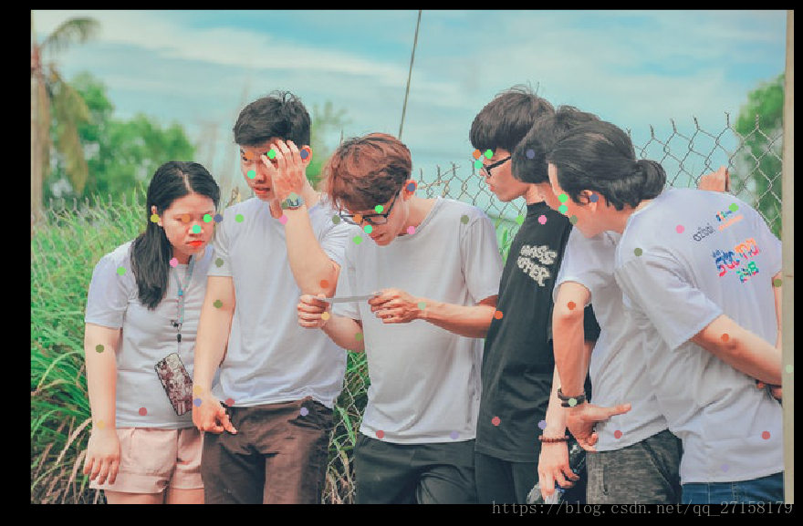
圖6. 在輸入圖片中顯示檢測到的關鍵點。

也可以不在輸入圖片中顯示關鍵點。

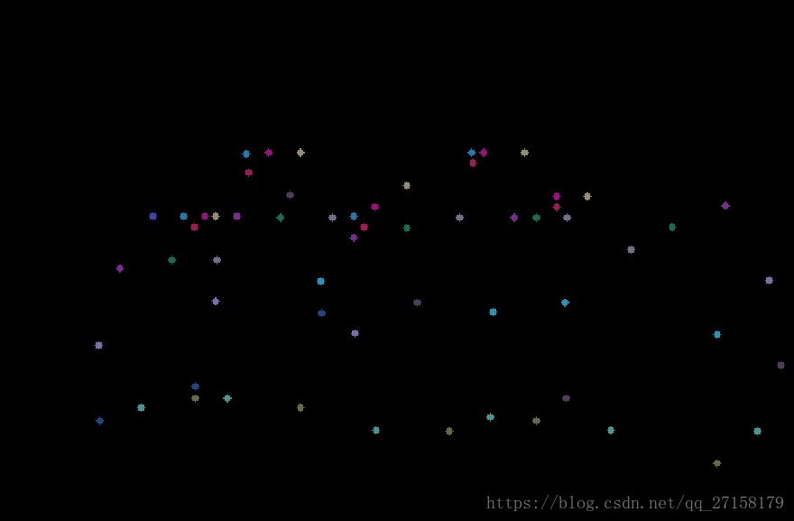
圖7. 在黑背景中顯示檢測到的關鍵點

圖6中，可看全部關鍵點都找到了。但是，當關鍵點不在原圖上顯示（圖7），我們難以辨別關鍵點是屬於哪個人體的。我們必須魯棒性地實現關鍵點到人體的對映。這部分是很重要的同時實現起來容易出錯。為了實現對映，我們找到關鍵點的有效連線，然後把這些連線組合起來建立每個人體的骨骼。

5. 第三步：找到有效的連線對

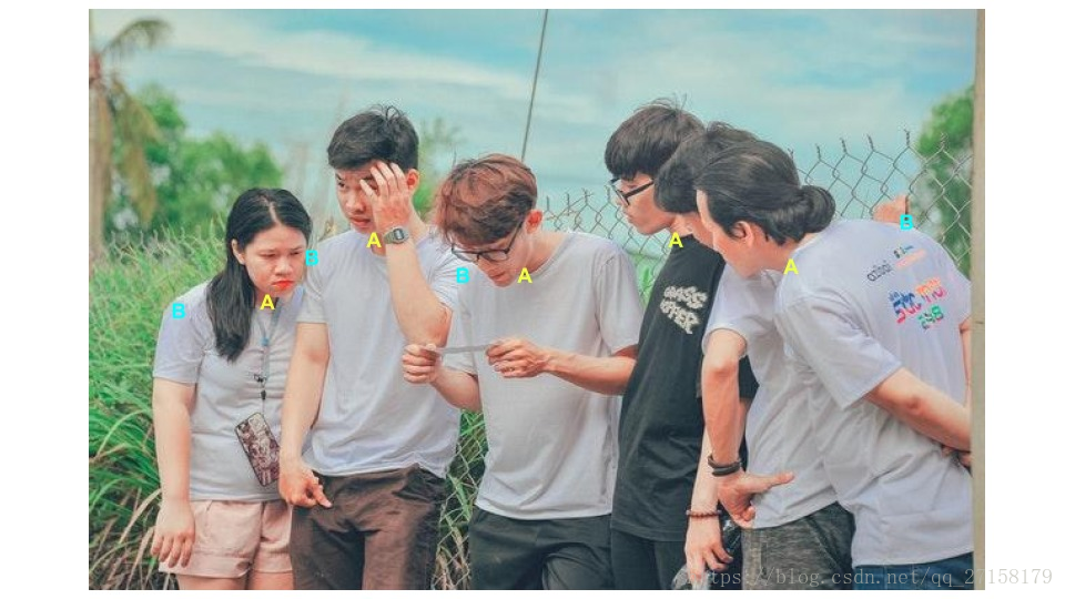
一個有效的連線對就是兩個關鍵點都在同一個人的人體部位上。一個最簡單的算出全部有效對方法就是找出一個關節到其他全部關節的最小距離。舉個例子，下圖中，我們可以找到標記好的鼻子到其他所有脖子的距離。最短距離那一對就是屬於同一個人的一對。

圖8. 使用測量距離得到關鍵點的連線

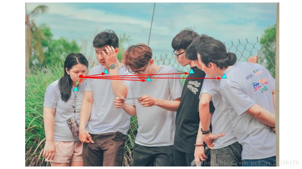
這個方法或者不是用於全部的連線對，特別是當圖中有很多人或者人與人之間有重疊。例如，在圖中左數起第二個人的左肘和左手腕的配對中，當這個人的左手肘和他本人的左手腕和第三個人的左手腕的距離相同，則無法用這個方法得到有效連線對。

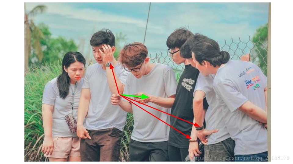
圖9. 只使用關鍵點之間的最小距離可能出現連線失敗

這部分就是部分親和圖開始發揮作用的地方。演算法給出了兩個節點對之間的親和性的方向。因此，一對關鍵點不僅具有最小距離，而且兩者的方向應該也符合PAF熱圖的方向。 （譯者注：這段話不容易翻譯，故給出了原文。This is where the Part Affinity Maps come into play. They give the direction along with the affinity between two joint pairs. So, the pair should not only have minimum distance, but their direction should also comply with the PAF Heatmaps direction.）

下圖是左手肘和左手腕連線的熱圖（Heatmap）。

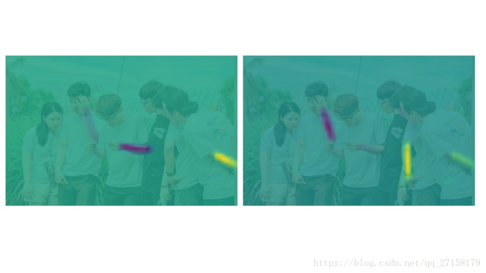
圖10. 左手肘-左手腕連線對的部分親和熱圖 因此，這個場合中，即使通過距離檢測法錯誤的識別連線對，由於PAF只同意連線第二個人的手肘和手腕的單位向量，所以OpenPose會輸出正確結果。

本方法在本文是這樣實現的：

1. 分割一條由兩個關鍵點組合成的線。找到這條線上的“n”個點。
2. 檢查PAF在這些點上的方向是否和連線這些點的線具有相同的方向。
3. 如果這個方向符合到了一定程度，則是有效的對。

在程式碼上看看這是如何實現的。以下程式碼片段屬於所提供的程式碼裡的getValidPairs()函式。      對於每個身體部位連線對，我們做了以下幾點：1. 把連線對上的關鍵點提取出來。相同的關鍵點放一起，把關鍵點分開地方到兩個列表上（列表名為candA和candB）。在列表candA上的每一個點都會和列表candB上某些點連線。下圖展示了連線對脖子-右肩的candA和candB。

圖11. 匹配脖子->鼻子的候選 Python

pafA = output[0, mapIdx[k][0], :, :]
pafB = output[0, mapIdx[k][1], :, :]
pafA = cv2.resize(pafA, (frameWidth, frameHeight))
pafB = cv2.resize(pafB, (frameWidth, frameHeight))

# Find the keypoints for the first and second limb
candA = detected_keypoints[POSE_PAIRS[k][0]]
candB = detected_keypoints[POSE_PAIRS[k][1]]

c++

//A->B constitute a limb
cv::Mat pafA = netOutputParts[mapIdx[k].first];
cv::Mat pafB = netOutputParts[mapIdx[k].second];

//Find the keypoints for the first and second limb
const std::vector<KeyPoint>& candA = detectedKeypoints[posePairs[k].first];
const std::vector<KeyPoint>& candB = detectedKeypoints[posePairs[k].second];

2. 得到連線兩個候選點的單位向量。得到了所連線這兩個點的線的方向。

Python

d_ij = np.subtract(candB[j][:2], candA[i][:2])
norm = np.linalg.norm(d_ij)
if norm:
    d_ij = d_ij / norm

c++

std::pair<float,float> distance(candB[j].point.x - candA[i].point.x,candB[j].point.y - candA[i].point.y);

float norm = std::sqrt(distance.first*distance.first + distance.second*distance.second);

if(!norm){
    continue;
}

distance.first /= norm;
distance.second /= norm;

3. 在連線兩點的直線上建立一個10個插值點的陣列（這句話也是百度翻譯的。真通順……）。 Python

# Find p(u)
interp_coord = list(zip(np.linspace(candA[i][0], candB[j][0], num=n_interp_samples),
                        np.linspace(candA[i][1], candB[j][1], num=n_interp_samples)))
# Find L(p(u))
paf_interp = []
for k in range(len(interp_coord)):
    paf_interp.append([pafA[int(round(interp_coord[k][1])), int(round(interp_coord[k][0]))],
                       pafB[int(round(interp_coord[k][1])), int(round(interp_coord[k][0]))] ])

                       C++

//Find p(u)
std::vector<cv::Point> interpCoords;
populateInterpPoints(candA[i].point,candB[j].point,nInterpSamples,interpCoords);
//Find L(p(u))
std::vector<std::pair<float,float>> pafInterp;
for(int l = 0; l < interpCoords.size();++l){
    pafInterp.push_back(
        std::pair<float,float>(
            pafA.at<float>(interpCoords[l].y,interpCoords[l].x),
            pafB.at<float>(interpCoords[l].y,interpCoords[l].x)
        ));
}

4. 對這些點的PAF和單位向量d_ij用點乘運算。 Python

# Find E
paf_scores = np.dot(paf_interp, d_ij)
avg_paf_score = sum(paf_scores)/len(paf_scores)    

c++

std::vector<float> pafScores;
float sumOfPafScores = 0;
int numOverTh = 0;
for(int l = 0; l< pafInterp.size();++l){
    float score = pafInterp[l].first*distance.first + pafInterp[l].second*distance.second;
    sumOfPafScores += score;
    if(score > pafScoreTh){
        ++numOverTh;
    }
     
    pafScores.push_back(score);
}
 
float avgPafScore = sumOfPafScores/((float)pafInterp.size());

5. 如果這些點中有70%滿足標準，則把這一對當成有效。 Python

# Check if the connection is valid
# If the fraction of interpolated vectors aligned with PAF is higher then threshold -> Valid Pair  
if ( len(np.where(paf_scores > paf_score_th)[0]) / n_interp_samples ) > conf_th :
    if avg_paf_score > maxScore:
        max_j = j
        maxScore = avg_paf_score

c++

if(((float)numOverTh)/((float)nInterpSamples) > confTh){
    if(avgPafScore > maxScore){
        maxJ = j;
        maxScore = avgPafScore;
        found = true;
    }
}

6. 第四步：  組合所有屬於同一個人的關鍵點繪出骨骼圖

既然我們已經把全部的關鍵點組合成對了，我們可以把具有相同部位檢測候選的連線對組合成複數個人體的姿態。（原文是Now that we have joined all the keypoints into pairs, we can assemble the pairs that share the same part detection candidates into full-body poses of multiple people.）

我們來看看這是如何實現的。以下程式碼段來自附帶程式碼中的getPersonwiseKeypoints()函式。

1. 我們首先建立空列表，用來存放每個人的關鍵點（即關鍵部位）。然後我們遍歷每一個連線對，檢查連線對中的partA是否已經存在於任意列表之中。如果存在，那麼意味著這關鍵點屬於當前列表，同時連線對中的partB也同樣屬於這個人體。因此，把連線對中的partB增加到partA所在的列表。 Python

for j in range(len(personwiseKeypoints)):
    if personwiseKeypoints[j][indexA] == partAs[i]:
        person_idx = j
        found = 1
        break
 
if found:
    personwiseKeypoints[person_idx][indexB] = partBs[i]

   C++

for(int j = 0; !found && j < personwiseKeypoints.size();++j){
    if(indexA < personwiseKeypoints[j].size() &&
       personwiseKeypoints[j][indexA] == localValidPairs[i].aId){
        personIdx = j;
        found = true;
    }
}/* j */
 
if(found){
    personwiseKeypoints[personIdx].at(indexB) = localValidPairs[i].bId;
}    

    2. 如果partA不存在於任意列表，那麼說明這一對屬於一個還沒建立列表的人體，於是需要新建一個新列表。

Python

# if find no partA in the subset, create a new subset
elif not found and k < 17:
    row = -1 * np.ones(19)
    row[indexA] = partAs[i]
    row[indexB] = partBs[i]

     c++  

else if(k < 17){
    std::vector<int> lpkp(std::vector<int>(18,-1));
 
    lpkp.at(indexA) = localValidPairs[i].aId;
    lpkp.at(indexB) = localValidPairs[i].bId;
     
    personwiseKeypoints.push_back(lpkp);
}

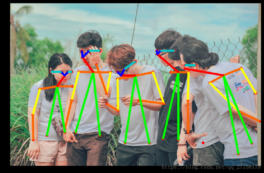
7. 結果

我們遍歷每個人並在輸入原圖上繪製骨架。 Python：

for i in range(17):
    for n in range(len(personwiseKeypoints)):
        index = personwiseKeypoints[n][np.array(POSE_PAIRS[i])]
        if -1 in index:
            continue
        B = np.int32(keypoints_list[index.astype(int), 0])
        A = np.int32(keypoints_list[index.astype(int), 1])
        cv2.line(frameClone, (B[0], A[0]), (B[1], A[1]), colors[i], 2, cv2.LINE_AA)
 
 
cv2.imshow("Detected Pose" , frameClone)
cv2.waitKey(0)

c++  

for(int i = 0; i< nPoints-1;++i){
    for(int n  = 0; n < personwiseKeypoints.size();++n){
        const std::pair<int,int>& posePair = posePairs[i];
        int indexA = personwiseKeypoints[n][posePair.first];
        int indexB = personwiseKeypoints[n][posePair.second];
 
        if(indexA == -1 || indexB == -1){
            continue;
        }
 
        const KeyPoint& kpA = keyPointsList[indexA];
        const KeyPoint& kpB = keyPointsList[indexB];
 
        cv::line(outputFrame,kpA.point,kpB.point,colors[i],2,cv::LINE_AA);
         
    }
}
 
cv::imshow("Detected Pose",outputFrame);
cv::waitKey(0);

下圖展示了每一個檢測到的人的骨架。

請自行執行程式碼驗證一下。

以上就是原文翻譯的內容。本文翻譯自https://www.learnopencv.com/multi-person-pose-estimation-in-opencv-using-openpose/ 原標題是Multi-Person Pose Estimation in OpenCV using OpenPose

至於原始碼，請自行上網站https://www.learnopencv.com/multi-person-pose-estimation-in-opencv-using-openpose/ 獲取。平時有逛learnopencv的讀者都知道，程式碼都託管在github上面的。所以獲取程式碼並不困難。我也不在這裡直接貼出連結了。