強烈建議先看 5.7 節，哈哈！

1 Tensorflow 簡介

1.1 科普: 人工神經網路 VS 生物神經網路

兩者的區別

人工神經網路靠的是正向和反向傳播來更新神經元, 從而形成一個好的神經系統, 本質上, 這是一個能讓計算機處理和優化的數學模型.
而生物神經網路是通過刺激, 產生新的聯結, 讓訊號能夠通過新的聯結傳遞而形成反饋.

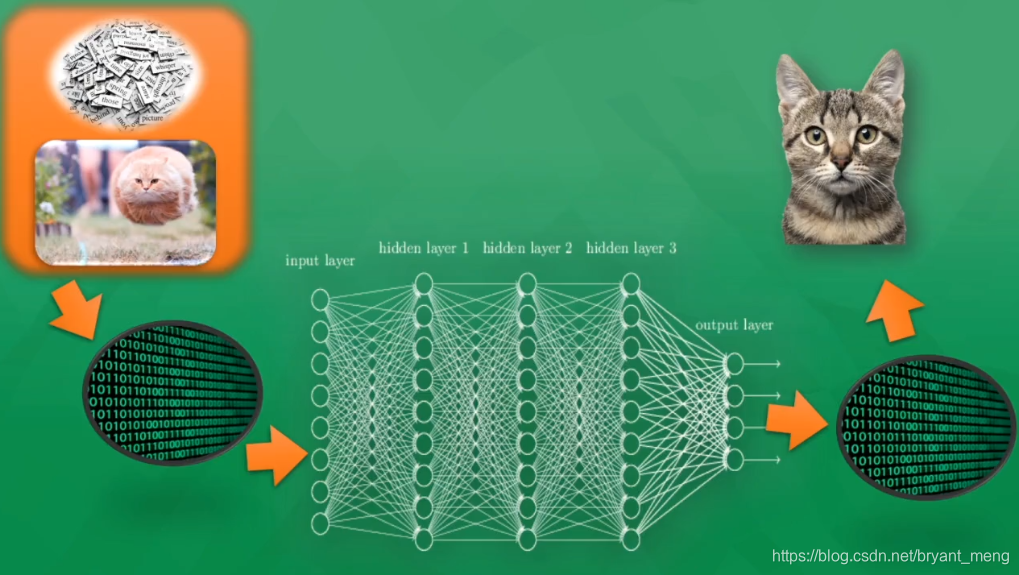
1.2 什麼是神經網路（機器學習）

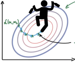
1.3 Gradient Descent in Neural Nets

Optimization family：Newton’s method、Gradient Descent、Least Squares method

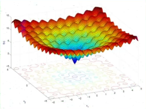
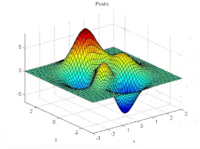
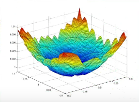
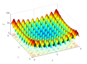
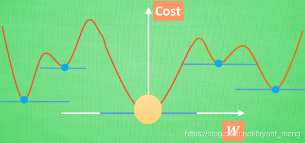
全域性最優固然是最好, 但是很多時候, 你手中的都是一個區域性最優解, 這也是無可避免的. 不過你可以不必擔心, 因為雖然不是全域性最優, 但是神經網路也能讓你的區域性最優足夠優秀, 以至於即使拿著一個區域性最優也能出色的完成手中的任務.

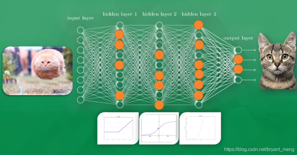
1.4 科普：神經網路的黑盒不黑

一層層照亮
與其說黑盒是在加工處理, 還不如說是在將一種代表特徵 (feature representation) 轉換成另一種代表特徵, 一次次特徵之間的轉換, 也就是一次次的更有深度的理解.

遷移

對於一個有分類能力的神經網路, 有時候我們只需要這套神經網路的理解能力, 並拿這種能力去處理其他問題. 所以我們保留它的代表特徵轉換能力

. 因為有了這種能力, 就能將複雜的圖片畫素資訊轉換成更少量, 但更精闢的資訊, 比如剛剛我們說將手寫數字變成的3個點資訊. 然後我們需要乾點壞事, 將這個神經網路的輸出層給拆掉. 套上另外一個神經網路, 用這種移植的方式再進行訓練, 讓它處理不同的問題, 比如, 預測照片裡事物的價值.

1.5 為什麼選 Tensorflow?

TensorFlow是Google開發的一款神經網路的Python外部的結構包, 也是一個採用資料流圖來進行數值計算的開源軟體庫.TensorFlow 讓我們可以先繪製計算結構圖, 也可以稱是一系列可人機互動的計算操作, 然後把編輯好的Python檔案轉換成更高效的C++, 並在後端進行計算

我覺得咯，社群大。

1.6 TensorFlow 的安裝

1.7 神經網路在幹嘛

擬合輸出

2 TensorFlow 基本框架

2.1 處理結構

2.2 y = k*x + b

import os  
  
os.environ["CUDA_DEVICE_ORDER"]="PCI_BUS_ID"   
os.environ["CUDA_VISIBLE_DEVICES"]="0,1"

控制使用哪個gpu，0 是0號卡，1是1號卡

import tensorflow as tf
import numpy as np

# create data
x_data = np.random.rand(100).astype(np.float32) # 隨機產生0-1直接的數
y_data = x_data*0.1 + 0.3
### create tensorflow sturcture start # 
Weight = tf.Variable(tf.random_uniform([1],-1.0,1.0)) # -1到1的某個數
bias = tf.Variable(tf.zeros([1]))

y = Weight * x_data + bias

loss = tf.reduce_mean(tf.square(y-y_data)) # 損失函式
optimizer = tf.train.GradientDescentOptimizer(0.5) # learning rate，優化方法
train = optimizer.minimize(loss) # 訓練

# init = tf.initialize_all_variables() # tf 馬上就要廢棄這種寫法
init = tf.global_variables_initializer()  # 替換成這樣就好
### create tensorflow sturcture end # 

with tf.Session() as sess:
    sess.run(init) # very important
    for step in range(201):
        sess.run(train)
        if step % 20 == 0:
            print(step,sess.run(Weight),sess.run(bias))

output

0 [-0.33800653] [0.6724009]
20 [-0.02264411] [0.36023486]
40 [0.06993133] [0.3147678]
60 [0.09262804] [0.30362064]
80 [0.09819263] [0.30088767]
100 [0.09955689] [0.30021766]
120 [0.09989133] [0.3000534]
140 [0.09997337] [0.3000131]
160 [0.09999347] [0.30000323]
180 [0.09999841] [0.3000008]
200 [0.09999961] [0.3000002]

2.3 Session 會話控制

以矩陣相乘為例，先來一個 numpy 版本

import numpy as np
matrix1 = np.mat([[3,3]])
matrix2 = np.mat([[2],
                 [2]])
product = np.dot(matrix1,matrix2)
print(product)

output

[[12]]

再來個 tensorflow 版本，Session 的第一種方式

import os  
import tensorflow as tf

matrix1 = tf.constant([[3,3]]) # 1,2
matrix2 = tf.constant([[2],
                       [2]])# 2,1
product = tf.matmul(matrix1,matrix2) # matrix multiply np,dot(m1,m2)

# method 1
sess = tf.Session()
result = sess.run(product)
print(result)
sess.close()

output

[[12]]

再來個 tensorflow 版本，Session 的第二種方式

import os  
import tensorflow as tf

matrix1 = tf.constant([[3,3]]) # 1,2
matrix2 = tf.constant([[2],
                       [2]])# 2,1
product = tf.matmul(matrix1,matrix2) # matrix multiply np,dot(m1,m2)

# method 2 
with tf.Session() as sess:
    result2 = sess.run(product)
    print(result)

output

[[12]]

2.4 Variable 變數

如果你在 Tensorflow 中設定了變數，那麼初始化變數是最重要的！！所以定義了變數以後, 一定要定義 init = tf.initialize_all_variables() 或者 init = tf.global_variables_initializer()

import tensorflow as tf
state = tf.Variable(0,name='counter')
#print(state.name)
one = tf.constant(1)
new_value = tf.add(state,one) # 變數+常量還是變數
update = tf.assign(state,new_value) 

init = tf.initialize_all_variables() # must have if define varible

with tf.Session() as sess:
    sess.run(init)
    for _ in range(3):
        sess.run(update)
        print(sess.run(state))
        #print(sess.run(update)) # 上面兩句等價於這一句

output

1
2
3

2.5 Placeholder 傳入值

placeholder 是 Tensorflow 中的佔位符，暫時儲存變數.
Tensorflow 如果想要從外部傳入data, 那就需要用到 tf.placeholder(), 然後以這種形式傳輸資料 sess.run(***, feed_dict={input: **}).

import tensorflow as tf
input1 = tf.placeholder(tf.float32)
input2 = tf.placeholder(tf.float32)

output = tf.multiply(input1,input2)

with tf.Session() as sess:
    print(sess.run(output,feed_dict={input1:7,input2:2.0})) #feed_dict 和 placeholder繫結
    #print(sess.run(output,feed_dict={input1:[7],input2:[2.0]}))

output

14.0

2.6 Activation Function

linear（直的）→ nolinear（掰彎）

deserialize(…)
elu(…): Exponential linear unit.
get(…)
hard_sigmoid(…): Hard sigmoid activation function.
linear(…)
relu(…): Rectified Linear Unit.
selu(…): Scaled Exponential Linear Unit (SELU).
serialize(…)
sigmoid(…)
softmax(…): Softmax activation function.
softplus(…): Softplus activation function.
softsign(…): Softsign activation function.
tanh(…)

3 構造我們第一個神經網路

3.1 新增層 def add_layer()

在 Tensorflow 裡定義一個新增層的函式可以很容易的新增神經層,為之後的新增省下不少時間.

import tensorflow as tf
import numpy as np
def add_layer(inputs,in_size,out_size,activation_function=None):
    Weights = tf.Variable(tf.random_normal([in_size,out_size]))#Outputs random values from a normal distribution
    bias = tf.Variable(tf.zeros([1,out_size])+0.1)
    Wx_plus_b = tf.matmul(inputs,Weights)+bias
    if activation_function is None:
        outputs = Wx_plus_b
    else:
        outputs = activation_function(Wx_plus_b)
    return outputs

output

3.2 建造神經網路

資料視覺化如下

三層，input layer 1 ， hidden layer 10 ， output 1

# Make up some real data
x_data = np.linspace(-1,1,300)[:,np.newaxis] #(300,1)
noise = np.random.normal(0,0.05,x_data.shape) # (300,1)
y_data = np.square(x_data)-0.5 + noise # (300,1)

# define placeholder for inputs to network
xs = tf.placeholder(tf.float32,[None,1])
ys = tf.placeholder(tf.float32,[None,1])
# add hidden layer
l1 = add_layer(xs,1,10,activation_function=tf.nn.relu) # hidden layer
# add ouput layer
prediction = add_layer(l1,10,1,activation_function=None) # output layer
# the error between prediction and real data
loss = tf.reduce_mean(tf.reduce_sum(tf.square(ys-prediction),
                                    reduction_indices=[1]))# 求和求平均，不要tf.reduce_sum結果也一樣
train_step = tf.train.GradientDescentOptimizer(0.1).minimize(loss)

# important step
init = tf.global_variables_initializer()
sess = tf.Session()
sess.run(init)

for i in range(1000):
    sess.run(train_step,feed_dict={xs:x_data,ys:y_data})
    if i%100 == 0:
        print(sess.run(loss,feed_dict={xs:x_data,ys:y_data}))
        #prediction_value = sess.run(prediction, feed_dict={xs: x_data})

output

1.2329736
0.004921457
0.0041357405
0.0037725214
0.0035861263
0.003505876
0.0034505243
0.00340674
0.0033686347
0.0033322722

loss 在漸漸下降

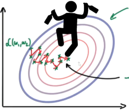
3.3 Speed Up Training

gradient descent 像喝醉酒一樣，搖搖晃晃，優化後，穩了

Stochastic Gradient Descent
With momentum
AdaGrad
RMSProp
Adam

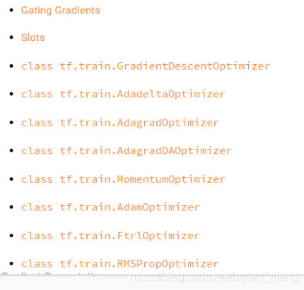
3.4 Optimizer

4 Tensorboard

在這裡插入圖片描述

4.1 GRAPHS

程式碼在3.1 和 3.2 節的基礎上添加了一些視覺化的程式碼
eg

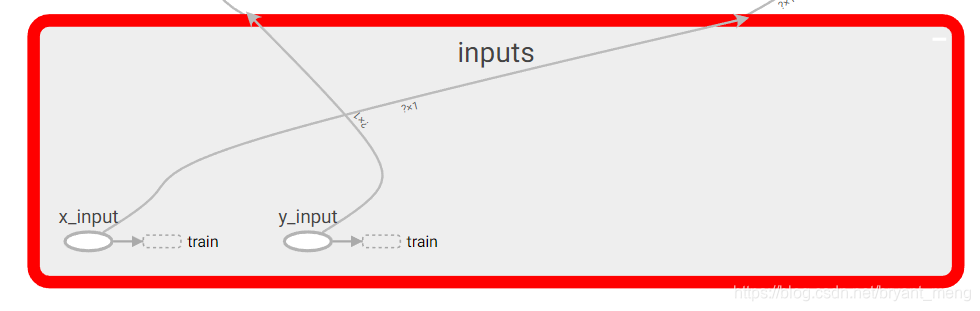
with tf.name_scope('inputs'): 
    xs = tf.placeholder(tf.float32,[None,1],name = 'x_input')
    ys = tf.placeholder(tf.float32,[None,1],name = 'y_input')

with tf.name_scope() 形成大的圖層

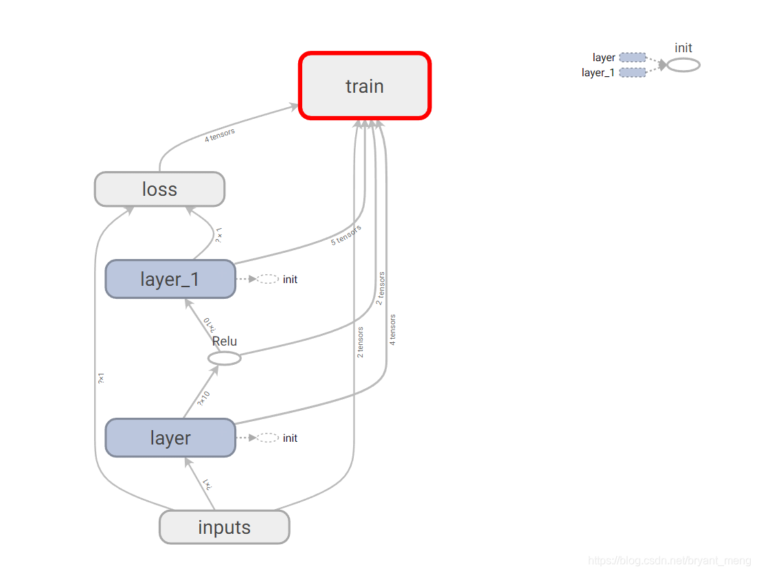
name 形成小元件，大圖雙擊就可以展開了

最後加上一句 畫龍點睛 writer = tf.summary.FileWriter("logs/", sess.graph) ，在當前目錄下建立logs資料夾，生成events.out.tfevents.xxxx 檔案，開 tensorboard 的時候把目錄指向 logs 即可

import tensorflow as tf
import numpy as np
def add_layer(inputs,in_size,out_size,activation_function=None):
    with tf.name_scope("layer"):
        with tf.name_scope("Weights"):
            Weight = tf.Variable(tf.random_normal([in_size,out_size]),name = "w")
        with tf.name_scope("bias"):
            bias = tf.Variable(tf.zeros([1,out_size])+0.1,name = "b")
        with tf.name_scope("Wx_b"):
            Wx_b = tf.add(tf.matmul(inputs,Weight),bias)
    if activation_function is None:
        outputs = Wx_b
    else:
        outputs = activation_function(Wx_b)
    return outputs

# Make up some real data
x_data = np.linspace(-1,1,300)[:,np.newaxis] #(300,1)
noise = np.random.normal(0,0.05,x_data.shape) # (300,1)
y_data = np.square(x_data)-0.5 + noise # (300,1)

# define placeholder for inputs to network
with tf.name_scope('inputs'):
    xs = tf.placeholder(tf.float32,[None,1],name = 'x_input')
    ys = tf.placeholder(tf.float32,[None,1],name = 'y_input')
# add hidden layer
l1 = add_layer(xs,1,10,activation_function=tf.nn.relu) # hidden layer
# add ouput layer
prediction = add_layer(l1,10,1,activation_function=None) # output layer
# the error between prediction and real data
with tf.name_scope("loss"):
    loss = tf.reduce_mean(tf.reduce_sum(tf.square(ys-prediction),
                                        reduction_indices=[1]))# 求和求平均，不要tf.reduce_sum結果也一樣
with tf.name_scope("train"):
    train_step = tf.train.GradientDescentOptimizer(0.1).minimize(loss)

# important step
init = tf.global_variables_initializer()
sess = tf.Session()
sess.run(init)
writer = tf.summary.FileWriter("logs/", sess.graph)

for i in range(1000):
    sess.run(train_step,feed_dict={xs:x_data,ys:y_data})

可以右鍵選擇把 train ，remove from main graph

4.2 DISTRIBUTION and HISTOGRAMS

看 Weight，bias，outputs 的 distribution 和 histograms 是用如下語句

tf.summary.histogram(layer_name, Weight)
tf.summary.histogram(layer_name, bias)
tf.summary.histogram(layer_name, outputs)

看 loss 是用

tf.summary.scalar('loss', loss) # tensorflow >= 0.12 新增

畫龍點睛為

merged = tf.summary.merge_all() # tensorflow >= 0.12 新增

merged 的後期處理看詳細程式碼，在 4.1 的基礎上加了上述程式碼

import tensorflow as tf
import numpy as np
def add_layer(inputs,in_size,out_size,n_layer,activation_function=None): # 新增了 n_layer 方便命名
    layer_name = "layer%s"%n_layer # 新增
    with tf.name_scope(layer_name):
        with tf.name_scope("Weights"):
            Weight = tf.Variable(tf.random_normal([in_size,out_size]),name = "w")
            tf.summary.histogram(layer_name, Weight) # 新增
        with tf.name_scope("bias"):
            bias = tf.Variable(tf.zeros([1,out_size])+0.1,name = "b")
            tf.summary.histogram(layer_name, bias)     # 新增
        with tf.name_scope("Wx_b"):
            Wx_b = tf.add(tf.matmul(inputs,Weight),bias)
    if activation_function is None:
        outputs = Wx_b
    else:
        outputs = activation_function(Wx_b)
    tf.summary.histogram(layer_name + '/outputs', outputs)      # 新增
    return outputs

# Make up some real data
x_data = np.linspace(-1,1,300)[:,np.newaxis] #(300,1)
noise = np.random.normal(0,0.05,x_data.shape) # (300,1)
y_data = np.square(x_data)-0.5 + noise # (300,1)

# define placeholder for inputs to network
with tf.name_scope('inputs'):
    xs = tf.placeholder(tf.float32,[None,1],name = 'x_input')
    ys = tf.placeholder(tf.float32,[None,1],name = 'y_input')
# add hidden layer
l1 = add_layer(xs,1,10,activation_function=tf.nn.relu,n_layer = 1) # hidden layer
# add ouput layer
prediction = add_layer(l1,10,1,activation_function
              
           
              
              
            
            相關推薦
			   
            
            
            
 

    

    
    《Tensorflow | 莫煩 》learning notes
      
							
							
							
強烈建議先看 5.7 節，哈哈！



1 Tensorflow 簡介
1.1 科普: 人工神經網路 VS 生物神經網路
兩者的區別


人工神經網路靠的是正向和反向傳播來更新神經元, 從而形成一個好的神經系統, 本質上, 這是一個能讓計算機處理和優化的數學模 

  
 

    

    
    tensorflow 莫煩教程
      訓練   ali   為什麽   run   info   指定   形式   顯示   優化參數   1，感謝莫煩
2，第一個實例：用tf擬合線性函數

import tensorflow as tf
import numpy as np

# create data
x_data = np.random. 

  
 

    

    
    TensorFlow 莫煩視訊學習筆記例子二（一）
      
							
							
							註釋連結

所有程式碼

# -*- coding: utf-8 -*-
"""
Created on Wed Apr 19 12:30:49 2017

@author: lg

同濟大學B406
"""

import tensorflow as tf
im 

  
 

    

    
    莫煩tensorflow(8)-CNN
      eal   mage   glob   padding   have   mat   and   for   variable   import tensorflow as tffrom tensorflow.examples.tutorials.mnist import input_data#number  

  
 

    

    
    莫煩tensorflow(2)-Session
      ()   lose   imp   int   close   min   import   log   result   import os os.environ[‘TF_CPP_MIN_LOG_LEVEL‘]=‘2‘ 
import tensorflow as tfmatrix1 = tf.constan 

  
 

    

    
    莫煩大大TensorFlow學習筆記（3）----建立神經網絡
      nbsp   定義數據   學習筆記   variables   ati   選擇   mea   有變   plus   1、def add_layer()
添加神經網絡層：
 

import tensorflow as tf

def add_layer( inputs, in_size, out_si 

  
 

    

    
    莫煩大大TensorFlow學習筆記（4）----分類問題
      rop   entropy   cti   cross   tensor   mea   orf   code   edi   1、分類的loss損失函數：可設為交叉熵

cross_entropy = tf.reduce_mean( -tf.reduce_sum ( ys * tf.log ( predic 

  
 

    

    
    莫煩大大TensorFlow學習筆記（5）----優化器
      一、TensorFlow中的優化器 
tf.train.GradientDescentOptimizer：tf.train.AdadeltaOptimizertf.train.AdagradOptimizertf.train.AdagradDAOptimizertf.train.MomentumOptimiz 

  
 

    

    
    莫煩大大TensorFlow筆記（6）----結果可視化
      tput   optimize   第一次   mage   orf   .sh   class   sum   nbsp   
#import os
#os.environ[‘TF_CPP_MIN_LOG_LEVEL‘] = ‘2‘
import tensorflow as tf
import nu 

  
 

    

    
    深度學習視訊，吳恩達，CS231n，斯坦福，計算機視覺，牛津大學，xDeepMind ，自然語言處理，莫煩，Tensorflow
       
 
 1. 吳恩達 最新深度學習視訊  網易雲課堂
 http://mooc.study.163.com/smartSpec/detail/1001319001.htm
 
 《深度學習筆記v5.32》 pdf下載
 連結:https://pan.baidu.com/s/1m8c7OdCJJZ2 

  
 

    

    
    莫煩python|Tensorflow筆記--tf10、tf11
      
                為神經網路新增一個神經層

import tensorflow as tf

# 新增一個神經層，定義新增神經層的函式
def add_layer(inputs, in_size, out_size, activation_function=None):
    Weight 

  
 

    

    
    莫煩python|Tensorflow筆記--什麼是迴圈神經網路RNN
      
                

我們在想象現在有一組資料序列，Data0，Data1,Data2,Data3，預測Results0的時候基於Data0，同意在預測其他結果的時候也是基於其他的數字。每次使用的神經網路都是同一個NN。如果這些資料是有關聯順序的，那麼就要遵從它們之間的順序，否則就串位了。但是 

  
 

    

    
    莫煩TensorFlow教程學習（1）
      
							
							
							第一次寫部落格真的是困難重重，心塞。。。

學習前的準備
環境準備：TensorFlow1.3.0+anaconda+python3.6.1

線性網路學習
（對應莫煩老師視訊教程的 ——例子2，此處放上原視訊連結本次學習視訊地址本次學習視訊連結（莫煩老師Ten 

  
 

    

    
    莫煩TensorFlow教程學習（4）——placeholder佔位符
      
								
								            
							
							
							
#莫煩TensorFlow教程學習

#placeholder(佔位符）傳入值學習 2018.10.10

import tensorflow as tf

#申明float32型別的placehol 

  
 

    

    
    深度學習(莫煩 神經網路 lecture 4） TensorFlow （GAN）
      
							
							
							



TensorFlow （GAN）



目錄






1、GAN

今天我們會來說說現在最流行的一種生成網路, 叫做 GAN, 又稱生成對抗網路, 也是 Generative Adversarial Nets 的簡稱



1.1 常見神經網路形式
 

  
 

    

    
    稍稍亂入的CNN，本文依然是學習周莫煩視頻的筆記。
      inpu   nec   real   data   tutorials   輸入   res   print   urn   　　稍稍亂入的CNN，本文依然是學習周莫煩視頻的筆記。　　　　還有 google 在 udacity 上的 CNN 教程。　　　　CNN(Convolutional Neural N 

  
 

    

    
    莫煩課程Batch Normalization 批標準化
      github   cti   mas   pen   get   lin   pytorch   生成   def   
 for i in range(N_HIDDEN):               # build hidden layers and BN layers
            input 

  
 

    

    
    莫煩TensorFlow_08 tensorboard可視化進階
      post   init   orm   ssi   rain   desc   light   rap   graph   
import tensorflow as tf  
import numpy as np  
import matplotlib.pyplot as plt  
  
 #
 # ad 

  
 

    

    
    莫煩TensorFlow_07 tensorboard可視化
      nbsp   des   edi   reduce   put   puts   lac   瀏覽器   between   
import tensorflow as tf  
import numpy as np  
import matplotlib.pyplot as plt  
  
def add 

  
 

    

    
    莫煩TensorFlow_11 MNIST優化使用CNN
      UNC   com   tutorials   optimizer   卷積   func   mea   cas   softmax   
import tensorflow as tf
from tensorflow.examples.tutorials.mnist import input_data

《Tensorflow | 莫煩 》learning notes

1 Tensorflow 簡介

1.1 科普: 人工神經網路 VS 生物神經網路

1.2 什麼是神經網路（機器學習）

1.3 Gradient Descent in Neural Nets

1.4 科普：神經網路的黑盒不黑

1.5 為什麼選 Tensorflow?

1.6 TensorFlow 的安裝

1.7 神經網路在幹嘛

2 TensorFlow 基本框架

2.1 處理結構

2.2 y = k*x + b

2.3 Session 會話控制

2.4 Variable 變數

2.5 Placeholder 傳入值

2.6 Activation Function

3 構造我們第一個神經網路

3.1 新增層 def add_layer()

3.2 建造神經網路

3.3 Speed Up Training

3.4 Optimizer

4 Tensorboard

4.1 GRAPHS

4.2 DISTRIBUTION and HISTOGRAMS

相關推薦

《Tensorflow | 莫煩》learning notes