# -*-encoding: utf-8 -*-
"""
@version: 3.6
@time: 2018/4/16 22:45
@author: SunnyYang
"""
from __future__  import print_function

from time import time   #計算每個步驟花費多長時間
from matplotlib import pyplot as plt
import logging
from sklearn.model_selection import train_test_split
from sklearn.datasets import fetch_lfw_people
from sklearn.model_selection import GridSearchCV
from sklearn.metrics import classification_report
from sklearn.metrics import confusion_matrix
from sklearn.decomposition import RandomizedPCA
from sklearn.decomposition import PCA
from sklearn.svm import SVC
 

#列印輸出日誌資訊
logging.basicConfig(format='%(asctime)s : %(levelname)s : %(message)s', level=logging.INFO,filename='svmFaceRecongnize.log') #列印時間，日誌級別以及日誌資訊

#資料採集
lfw_people = fetch_lfw_people(min_faces_per_person=70,resize=0.2)   #fetch_lfw_people()用來下載名人資料

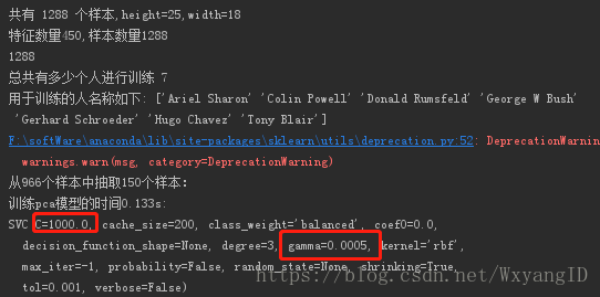
#資料預處理
n_samples, h, w = lfw_people.images.shape   #資料集共有多少個樣本，以及每一張圖片的high 和width
print('共有 %s 個樣本,height=%s,width=%s'%(n_samples,h,w))   #注意佔位符的使用是用%（）的形式，而不是每一個都用佔位符
X = lfw_people.data  #data屬性是取出所有特徵值，每一行是一個樣本，每一列是一個特徵
# e = X[0:5,:] #切片操作取出矩陣的0到5行，和所有列
# print(e)
n_features = X.shape[1]  # 450個特徵值，1表示的是列 0表示的是行數
n_sampless = X.shape[0]  #1288行 例項的個數
print('特徵數量%s,樣本數量%s'%(n_features,n_sampless))  #450,1288
y = lfw_people.target #每一個例項的類別標記
target_names = lfw_people.target_names  #提取不同人的身份，就是真實的名字是什麼
n_class = target_names.shape[0] #總共有多少個人=多少類=多少行進行人臉識別
print(len(y))
print('總共有多少個人進行訓練',n_class)
print('用於訓練的人名稱如下:',target_names)

#拆分成訓練集和測試集
x_train,x_test,y_train,y_test = train_test_split(X,y,test_size=0.25) #x_train,x_test是一個特徵矩陣，y_train,y_test是對應的標記向量
 

#資料降維及模型訓練
n_components = 150 #組成元素的數量，也就是降維後的維度
print('從%s個樣本中抽取%s個樣本：' %(x_train.shape[0],n_components))
t0 = time() #定義一個起始時間
pca = RandomizedPCA(n_components=n_components,whiten=True).fit(x_train)  #採用經典的pca主成分降維方法
# pca = PCA(svd_solver='ranomized',n_components=n_components,whiten=True).fit(x_train)  #
print('訓練pca模型的時間%0.3fs:'%(time()-t0))
eigenfaces = pca.components_.reshape((n_components,h,w)) #從一張人臉上提取一些特徵 ，對於人臉的一張照片上提取的特徵值名為eigenfaces
x_train_pca = pca.transform(x_train) #將訓練集中的所有特徵值通過pca轉換成低緯特徵量
x_test_pca = pca.transform(x_test) #同理將測試集也降維

#核函式的構造，c懲罰因子也有人說是權重，gamma是特徵值的對應的比例也就是有多少個特徵點被使用 ，引數中共有6*6=36中不同的組合
param_grid = {'C':[1e3,5e3,1e4,5e4,1e5,5e5],
              'gamma':[0.0001,0.0005,0.01,0.05,0.1,0.5]
              }
clf = GridSearchCV( SVC(kernel='rbf',class_weight='balanced'),param_grid) #將引數的各種組合均放到svc中進行計算，最後看哪一組引數的效果好
clf = clf.fit(x_train_pca,y_train) #建模，找到使得邊際最大的超平面
print(clf.best_estimator_) #列印輸出最好的模型所對應的引數
 

#預測
y_pred = clf.predict(x_test_pca)
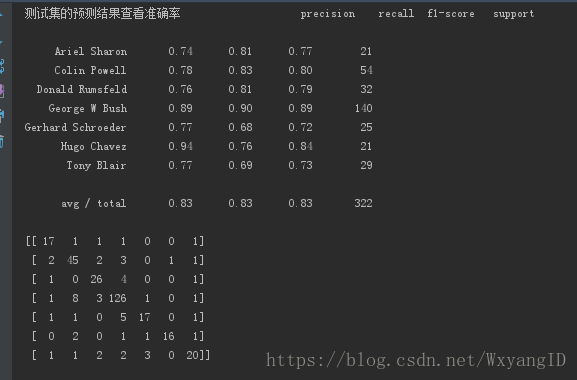
print('測試集的預測結果查看準確率',classification_report(y_test,y_pred,target_names=target_names)) #預測的準確率是多少
print(confusion_matrix(y_test,y_pred,labels=range(n_class))) #預測矩陣，對角線上的值越多，則說明預測的準確率越高，行和列分別是真實的和預測的標記，如果兩者相等則值加一，所以對角線上的值是最有效的

#視覺化預測結果和特徵矩陣
def plot_galley(images,titles,h,w,n_row=3,n_col=4):
    plt.figure(figsize=(1.8 * n_col,2.5 * n_row))
    plt.subplots_adjust(bottom=0,left=.01,right=.99,top=.90,hspace=.35)
    for i in range(n_row * n_col):
        plt.subplot(n_row,n_col,i+1) #subplot()三個引數，分別是幾行幾列子圖的位置在第幾個
        plt.imshow(images[i].reshape((h,w)),cmap=plt.cm.gray) #imshow()展示的是一個矩陣images重新按照h,w來重構，reshape是np中的一個數組重構的方法，cmap=colormap
        plt.title(titles[i],size=12)
        plt.xticks(())  #x軸刻度
        plt.yticks(())  #y軸刻度

def title(y_pred,y_test,target_names,i):
    pre_name = target_names[y_pred[i]].rsplit(' ',1)[-1]   #預測的名字
    true_name = target_names[y_test[i]].rsplit(' ',1)[-1]   #真實的名字
    return 'predict %s\ntrue    %s'%(pre_name,true_name)    #

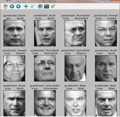
prediction_titles = [title(y_pred,y_test,target_names,i) for i in range(y_pred.shape[0])] #預測的人名字
plot_galley(x_test,prediction_titles,h,w)   #
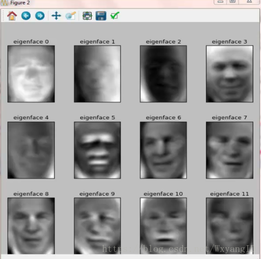
eigenface_titles = ['eigenface %d '% i for i in range(eigenfaces.shape[0])]     #
plot_galley(eigenfaces,eigenface_titles,h,w)  #提取的特徵向量組成的臉是什麼樣子的
plt.show()