Spain’s main economic aggregates forecasted using ARIMA

To begin with, I’d like to give a big shout out to Manos Antoniou for sharing his analysis of the the Eurozone’s GDP in this article. I was inspired by it and it motivated me to replicate and extend his analysis specifically for the country where I currently live, which is Spain. If you didn’t read his article, I encourage you to do it!

Following his blueprint, I’m going to do some time series modelling and forecasting using the information available at the Eurostat Database.

The Eurostat Database is a fantastic repository of economic statistics that can be consulted online, and luckily we also can do it directly from R!

Here’s how Eurostat

“Eurostat’s main role is to process and publish comparable statistical information at European level. We try to arrive at a common statistical ‘language’ that embraces concepts, methods, structures and technical standards.

Eurostat does not collect data. This is done in Member States by their statistical authorities. They verify and analyse national data and send them to Eurostat. Eurostat’s role is to consolidate the data and ensure they are comparable, using harmonized methodology. Eurostat is actually the only provider of statistics at European level and the data we issue are harmonized as far as possible.”

What I’m going to do is to download some data from Eurostat using the eurostat package in R, analyze the time series, model and forecast them the next 8 quarters for each of the following 6 aggregates:

1. GDP (gross domestic product at market prices)
2. Consumption (final consumption expenditure)
3. Gross Capital (gross capital formation)
4. Exports (of goods and services)
5. Imports (of goods and services)
6. Salaries (wages and salaries)

We will have 6 time series with quarterly frequency starting in 1995 and ending in Q2 2018.

We will do ARIMA modelling.

ARIMA model (Auto-Regressive Integrated Moving Average)

• In an auto-regressive model (AR) we forecast the variable of interest using a linear combination of past values of the variable
• In a moving average model (MA), rather than using past values of the forecast variable, we use past forecast errors
• ARIMA combines both auto-regressive models and moving average models, while also differencing the series (integrated in this context means the reverse of differencing) to deal with non-stationarity.
• Compared to exponential smoothing models, which are based on a description of the trend and seasonality in the data, ARIMA models aim to describe the auto-correlations in the data.

A seasonal ARIMA model includes seasonal terms. We will talk about an ARIMA(p,d,q)(P,D,Q)m model, where:

• p = order of the auto-regressive non-seasonal part
• d = degree of first differencing involved for the non-seasonal part
• q = order of the moving average non-seasonal part
• P = order of the auto-regressive seasonal part
• D = degree of first differencing involved for the seasonal part
• Q = order of the moving average seasonal part
• m = number of observations per year

Data acquisition & exploratory analysis

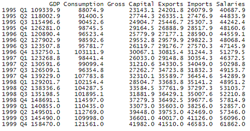
After using the eurostat API, downloading and importing the data (check the full R code for the details), we take a look at the fist and last rows:

head(data, 20)

tail(data, 20)

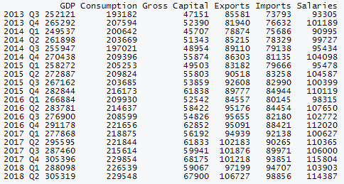
This is a plot of the 6 time series:

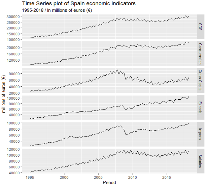
We will work on each of this time series one by one.

Let’s focus first on the GDP time series.

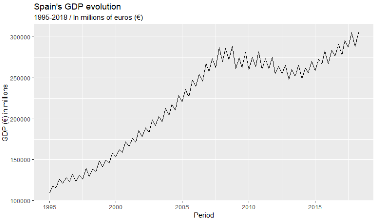
The GDP series shows an upwards trend and apparent seasonality.

We can check seasonality with two plots:

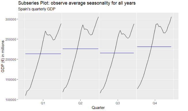
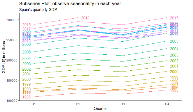
Both this plots allow us to understand that GDP behavior is seasonal, showing higher performance in Q2 and Q4 and lower in Q1 and Q3.

Modelling with ARIMA

To begin our modeling, we will first create a subset of the data in order to train the model and then be able to test its performance over unseen data (the data that we will purposefully hold out):

train_set <- window(data, end = c(2016, 4))

Then we use theauto.arima() function from the forecastpackage to fit an automatic ARIMA model:

arima_train <- auto.arima(train_set[, "GDP"],                           ic = "aicc",                           approximation = FALSE,                          stepwise = FALSE,                          lambda = "auto")

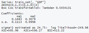
auto.arima() fits different models and selects ARIMA(0,1,2)(0,1,0)[4] as the best model.

Note: ARIMA uses maximum likelihood estimation (MLE). This means it finds the parameter values that maximize the probability of obtaining the data.

In order for this model to be acceptable we should see no pattern in normally-distributed residuals and it’s lags contained inside the ACF boundary. Let’s check it using checkresiduals()on our model object:

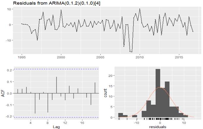
Residuals look indeed like white noise. We are good to go.

Let’s now check the performance of this model on the full data set, including the quarters we held out. We can calculate several accuracy scores at once:

round(accuracy(forecast(arima_train, h = 5), data[, "GDP"]), 3)

Among this accuracy metrics, we can look at MAPE (mean absolute percentage error). In this case, for the test set we score a MAPE of 1.7%. This is not extremely useful by itself, but it will help if we have several models we want to compare. Other than that, 1.7% seems a rather low error percentage and we will use this model to forecast.

We now proceed to extend the model to use all the available information (so as to take into consideration our most recent quarters, which were previously held out):

arima_full <- auto.arima(data[, "GDP"],                         ic = "aicc",                          approximation = FALSE,                         stepwise = FALSE,                         lambda = "auto")

This results again in our ARIMA(0,1,2)(0,1,0)[4] model.

We then use it to forecast the future 8 quarters and plot:

arima_full %>%  forecast(h = 8) %>%   autoplot() +   labs(title = "Spain's quarterly GDP forecast: ARIMA modelling",        subtitle = "In millions of euros (€), 2018-19",        y = "GDP (€)")+   scale_x_continuous(breaks = seq(1995, 2020, 1)) +   theme(axis.text.x = element_text(angle = 45, hjust = 1))

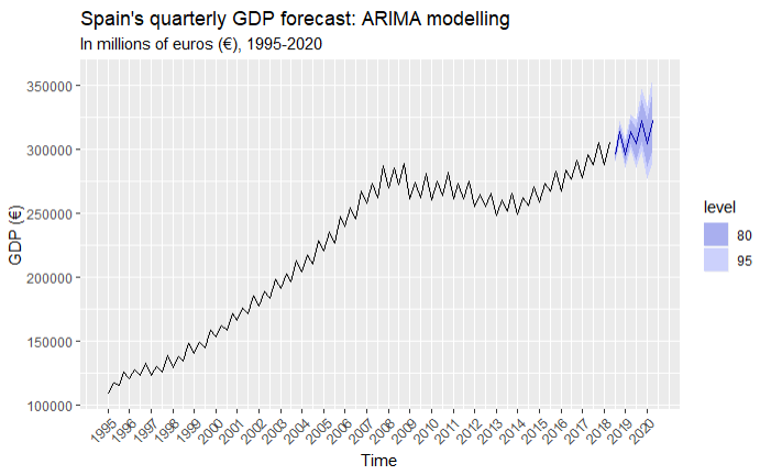
According to our forecast, Spain’s GDP for the next 8 quarters shows continuity of the upward trend while also correctly capturing seasonality. According to this projection, GDP at current prices will increase up to €326,293 million in the second quarter of 2020, which represents an increase of 6.87% against the same quarter of 2018 and an average increase of 0.86% per quarter.

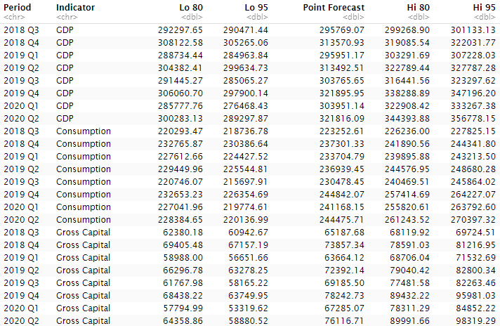
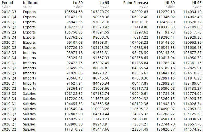
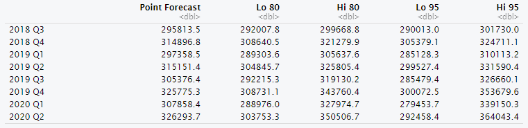
Here’s the complete forecast including confidence intervals:

Now we will proceed to replicate the same process for our other indicators. I will avoid technicalities and just plot the forecast and consolidate the numeric tables into one single table at the end.

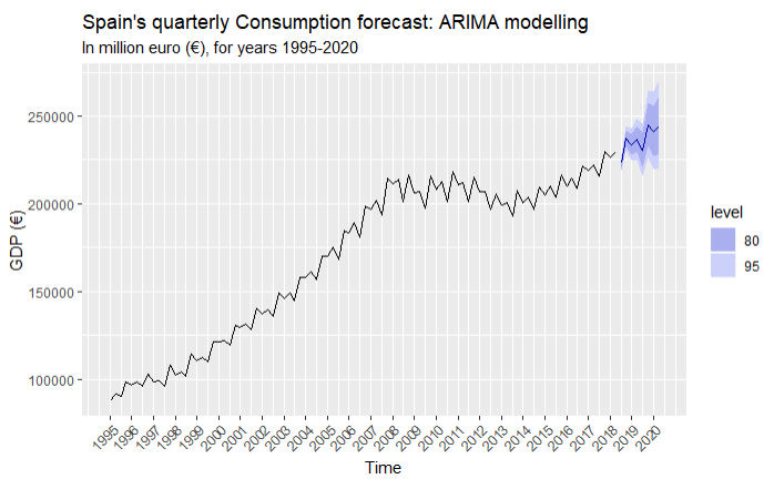
Consumption

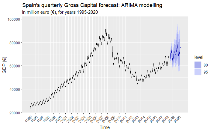
Gross Capital

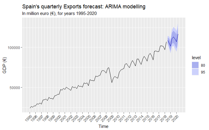
Exports

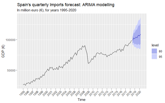
Imports

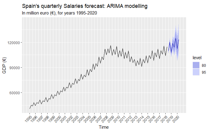
Salaries

Forecast summaries