Ever wanted to learn to use AWS, delve into genetics, or tinker with ML using python? If so, you’re in luck, because this tutorial is precisely about that! Specifically:

• Data-mining a raw 23andMe file for ancestry + unique traits
• Sweet visualisations using matplotlib/ wordcloud/ basemap/ geopy
• Dipping into ML with K-means + t-SNE dimensionality reduction
• Deploying on AWS using docker + the deploit platform

All this in ~100 lines of python. However for the impatient (wishing to keep under the promised 15 mins), source-code is available through

Disclaimers: A) Parts of the code have been adapted from online sources and the project relies on numerous open-source projects (refs appended).Thank you to these developers for making this project possible! B) The visualisations created are not meant to make factual/medical claims and should be interpreted as art rather than hard science — i.e. I am aware they are not fully rigorous in terms of genetics/statistics/ML

1) What we will create, and How

The script we will write takes 23andMe data (yours if you wish), and creates these neat visualisations:

• A word-cloud displaying traits associated with your genetic variations. That is, variations that might (emphasis on might) relate to aspects that make you …well: you.
• A plot of a world map, showing your estimated proportion of ancestry in certain ethnic groups
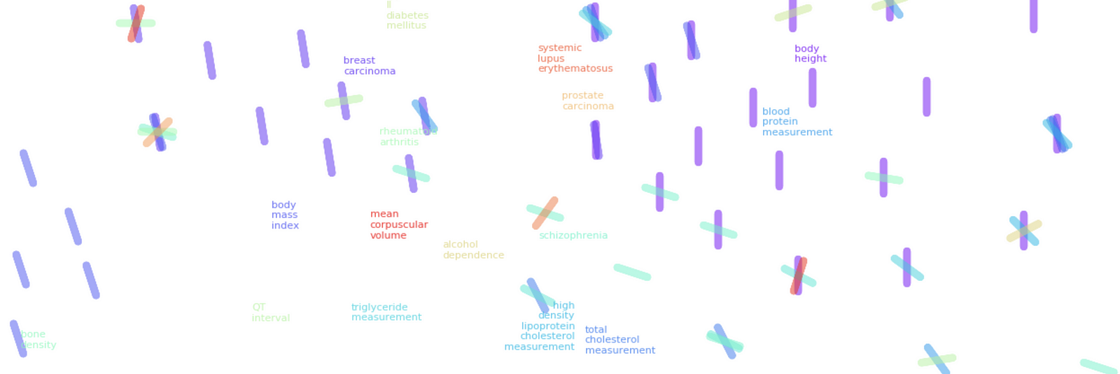
• A t-SNE dimensionality reduction graph of how your uncommon genetically-influenced traits cluster together.

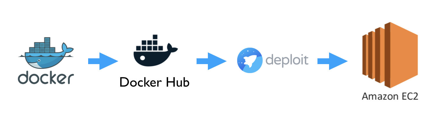
The code will be run in a docker container (think: lightweight VM), deployed on AWS using deploit bioinformatics platform (that retrieves the docker container from the Docker Hub repository — like GitHub for docker). Deploit allows for easy deployment of containers to Amazon EC2, and it is free for individual and community usage, i.e. you don’t pay a cent atm!

2) Download input data

Next, let’s retrieve two reference files and a sample 23andMe raw-data file. The 23andMe file consists of rows corresponding to genetic variations you express. These single-nucleotide polymorphisms (SNPs — pronounced ‘snips’) influence numerous individual traits. E.g. hair colour or your proclivity toward disliking cilantro. We will hence use this file to mine information about you (or an anonymous openSNP participant!). The three files we will need for the application are as follows:

1. A CSV file produced by the European Bioinformatics Institute, which records SNP-phenotype associations from thousands of studies. You can download it from here (untar it and call it refpanel_public_ref.gz).
2. A file for estimating your ancestry. Download it from here (rename it gwas_catalog.tsv)
3. A 23andMe file — you can download a sample 23andMe file from my GitHub repo.

Put all three files in the same folder. If you wish to use your own 23andMe data, replace the 23andme.txt with your own file.

3) Diving in! Writing the code

Now for the fun part. Start off by creating a folder named ‘geneticsdiy’ with three empty files: controller.py, Dockerfile (no file extension), and requirements.txt. Now open controller.py in an editor, and lets get to work. Here’s the whole file, which I will go through line-by-line:

Lines 1 to 18: importing all the goodies

Lines 21–48: the main function of the script, which imports the data, does the preprocessing, calls the ancestry.cpp function to find your ancestry, and calls the various image-creation functions.

Line 22: A list of file-names for convenient referencing.

Line 23: Using list comprehension, we rename the input files and copy them to the root of the docker container.

Lines 24 & 25: We gzip the 23andMe file (format required by the ancestry c++ executable).

Line 26: We use python’s subprocess.call method to call the ancestry estimation c++ module, which compares our DNA to that of numerous reference populations using probabilistic clustering (see Pritchard’s bitbucket for details). The output is a list of files names Test.*.Q, which we will retrieve to create the ancestry-map image. You can change the “2” to a higher number to make the estimate more accurate, but it will take longer to run.

Lines 27 & 31: We use the pandas module to read our reference and 23andMe files as spreadsheet-like DataFrame objects and rename some columns.

Lines 28–30: Remove non-numeric values, and select only SNP-phenotype association data in the reference file that has been found to be statistically significant, for SNPs that are uncommon in the population.

Line 32: Get rid of empty spaces between trait descriptions.

Lines 33–36: Assign a genetic variant column to our two DataFrame objects, which combines the SNP name, as well as which base-pair variant is actually the culprit in causing a given trait (reference DataFrame) vs. which ones you have inherited from your parents (23andMe DataFrame).

Lines 37 & 38: Find the intersection between the two DataFrames in terms of the columns we just created.

Lines 39 — 41: Change the chromosome column to be numeric instead of having ‘X’ and ‘Y’ as names.

Lines 42 & 43, 44 & 45: Use scikit learn’s K-means module to cluster SNPs by their chromosome and chromosome positions, then group all the associated traits of these clusters. The idea is that SNPs that influence the same gene are more likely to be in the same cluster.

Lines 46–48: Call the various image-creation functions. We pass the overlap functions for the word-cloud and cluster-visualisation functions. The latter also gets the cluster-grouped-associations array as an input parameter.

We’re half done! Now for the image-creation functions:

Lines 51–72: The function for creating the ancestry-map.

Lines 52–53: Dictionary of ancestry-group:location mappings, and initialising three empty dictionaries we will need.

Lines 54–58: Using python’s glob module, open all the Test.*.Q files produced by the ancestry c++ executable, recording the ancestry estimates from each file into our dictionary, along with their frequency.

Lines 59–62: Using the geopy module, we initialise a geo-location service provided by ArcGIS. We then take the mean of the ancestry estimates, and if the estimates proportion of ancestry is larger than 1%, we query ArcGIS for the latitude and longitude of the location we associate with that ancestry.

Lines 63- 66: We initialise basemap (which we will use to draw the map), and draw the continents, country-borders and background colours.

Lines 67–72: We iterate through the ancestry locations, annotating the map with numbers and disks corresponding to ancestry groups and their proportional contribution. Finally we save the image with high dpi as a png file.

Two thirds done!

Lines 77–82: The word-cloud. We initialise the pyplot figure (line 78), create a frequency list of SNP-traits from your list of variants (that we have filtered for p-value and rarity), create a new word-cloud object using the word-cloud python module, and save it as another png. That was easy!

Just one more function to go:

Lines 85–99: The SNP-cluster function.

Line 86: We create a list of the most common phenotypic traits in your data.

Line 87: We create a one-hot-encoding of how the various traits occur in our SNP-combined-clusters. That is, if a trait occurs in a cluster its column has a ‘1’; otherwise a ‘0’.

Line 88: We find the rows in which our most-common traits have a value of ‘1’ within the one-hot-encoding.

Line 89: We use Hinton’s t-SNE dimensionality reduction algorithm (using scikit learn’s TSNE module) to map this high-dimensional array into only two dimensions, where similar entries are close to each other in terms of Euclidean distance.

Lines 90–96: For each of the most common traits, we plot the t-SNE morphed coordinates of rows where the trait occurs. We do this with unique colors and marker-rotations for each trait to make things more interpretable, and annotate the name of the trait as well. The end result is a graph, where clusters of phenotypic traits lie closer to each other, with trait labels hovering at the mean coordinate around which it occurs in various trait clusters. I.e. if two trait names lie together, they tend to co-occur in your SNP clusters.

Lines 97–99: Finally, we use the adjust_text module to stop the annotations from overlapping too much, and save the figure and a png.

Lines 101–102: Make the script executable.

Done!!! From here it’s a breeze, I promise.

4) Deployment

A) Operation: Dockerize ALL the things

Next step: install docker. Then, create a repo on Docker Hub (instructions here) — be sure to make it public so its visible in the steps below. To bundle our code as a container, we will still need to quickly complete the two remaining files: Dockerfile and requirements.txt. The former specifies how to set up our container (for example downloading the ancestry.cpp code and other necessary packages). The latter is a list of python modules to be downloaded using pip within the container. You can copy the code for both here and here.

Now simply call (within the geneticsdiy folder) the following commands to log into your docker account, build the container, and push it to your Docker Hub repo:

docker login --username=usernamedocker build -t geneticsdiy .docker tag geneticsdiy username/repo_name:geneticsdiydocker push username/repo_name:geneticsdiy

Dockerisation complete!

B) Deploit this bad boy

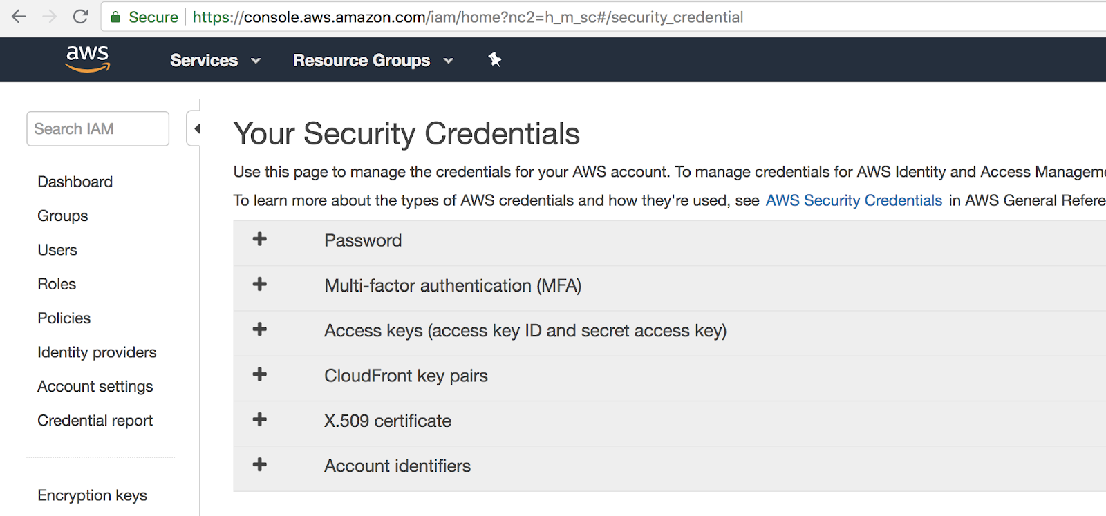
Lets take this doggo for a run. You’ll need an AWS account, and Amazon keys (credentials to interface with AWS programatically) to deploy on AWS; you can get them here (free account) and here.

Now, create a deploit account here. Once you’ve registered, go to your data-sets directory (bottom left), and add (using New → Import on the top right) a new data-set, with the 23andme.txt, refpanel_public_ref.gz, gwas_catalog.tsv files in the same data-set.

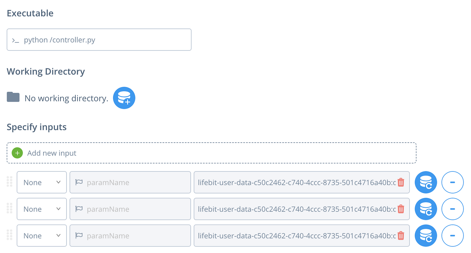
Let’s add our container as a pipeline. Proceed to the Pipeline section, and select New. Select the ‘docker’ option, and enter the details in the picture above (with your username and repo-name obviously). Click Create Pipeline. Now, go to the home-tab and click on the green rocket icon with ‘New’ on it. Select the geneticsdiy pipeline under ‘My Pipelines’. Add two extra parameters (+ symbol), set the left-most option to ‘None’ for each, and select the three input files (In the order seen in the pic below pls :O). Click next, create a new project to deploy it under (name it anything). Select an instance under Guaranteed Instances, to run it with (I recommend c3.xlarge under the CPUs = 4 category), and run the job. Nice, you’ve deployed the container on AWS!

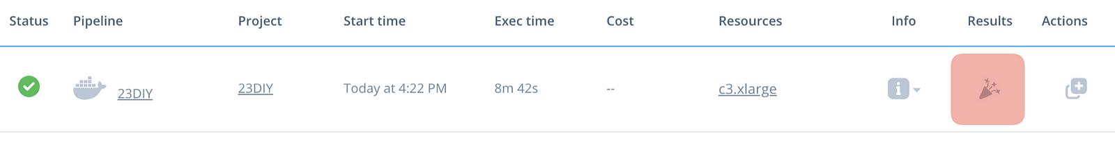
Wait for the job to get initialised (the status icon will turn blue — takes couple mins), then for it to run (will take ~10 mins). Once executed, click on the results button, which will take you to the data interface. Click on the results page to see the visualisations we have made.

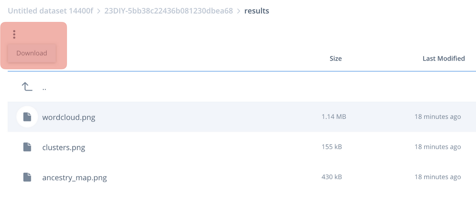
Woop! You’ve just obtained the processing results of your first cloud genetics app!

That wraps up our mini-project; I hope you have found this tutorial useful :)

Appendix: Thank you to these open-source projects, online answers, etc for making this tutorial possible:

1) Joe Pickrell’s ancestry C++ module. 2) European Bioinformatics Institute, 3) openSNP 4) Docker container with boost integration, 5) Deploit’s free offer, 6) Python wordcloud, geopy (and ArcGIS), basemap, adjustText modules 7) Numerous tutorials, 8) Anyone else I forgot — apologies!