Attention Model has been a rising star and a powerful model in the deep learning in recent years. Especially the concept of self attention proposed by Google in 2017, which can be applied to many fields as long as related to sequence. However, the knowledge gap between attention model and self attention has not been well explained, leading to the entry barrier for self attention. In this article, I will try to integrate the evolution of Machine Translation from

Seq2seq to attention model and to self attention.

This article is split into two parts. In the First part Seq2seq and Attention model are the main topic, whereas Self Attention will be in the second part.

Hope you enjoy it.

Preface

You might have heard Sequence-to-sequence(Seq2seq) model before, which is one of the most popular models nowadays. Seq2Seq is widely used for tasks such as machine translation, Chatbot/Q&A, caption generation and other cases where it is desirable to produce a sequence from another.

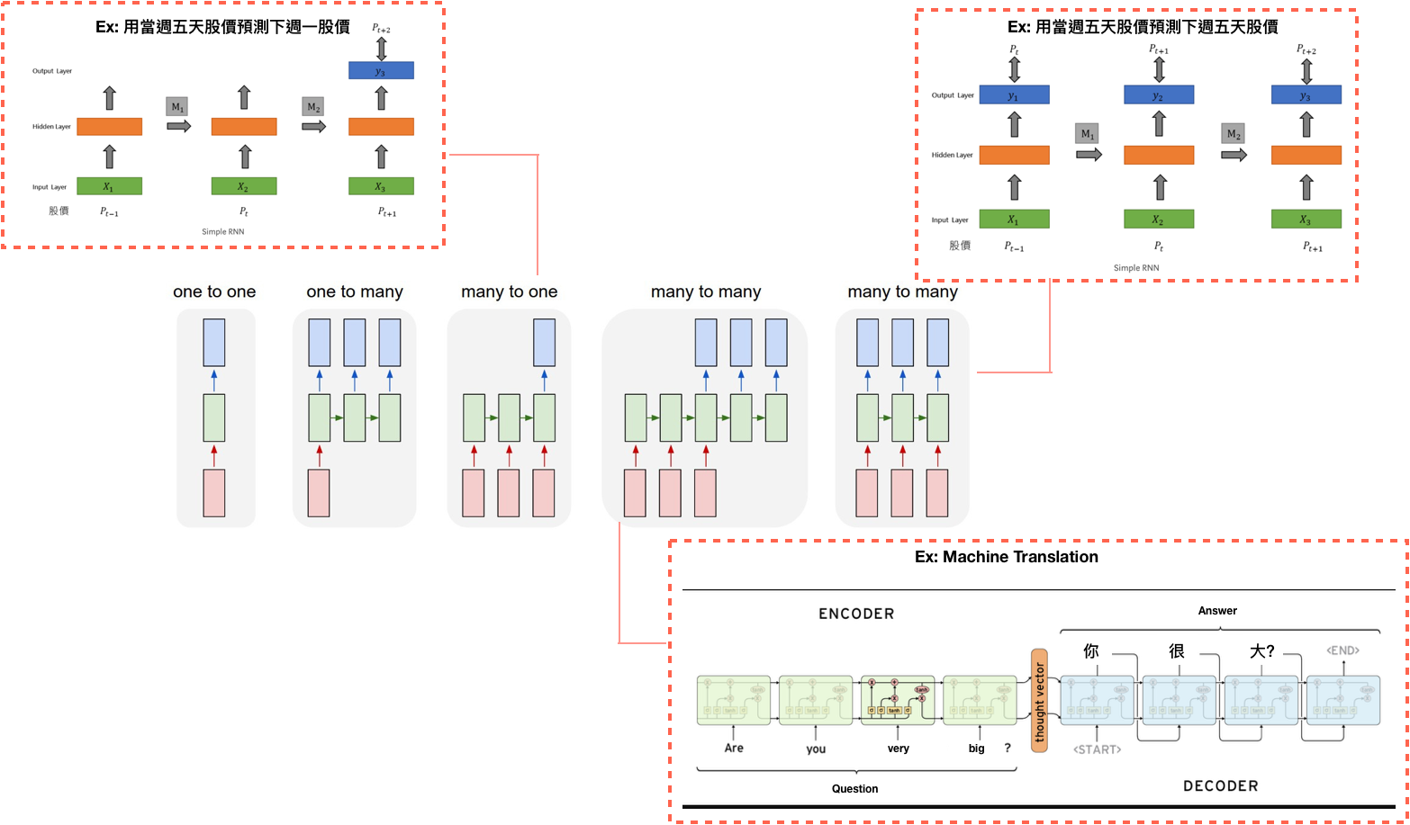
Let us take a look at some examples.

Since machine translation is in general use of Seq2seq model, we will use it as an instance in the upcoming paragraph.

Figure(3) is a classic Seq2seq model, which consists of Encoder and Decoder. Once inputing source into the encoder, you will get the target from the decoder.

For example, if we choose “Are you very big? ”as a source sentence, we will get “你很大？”as a target sentence. This is how machine translation works. However, looking at the formula on the right, we will find it’s easier said than done if we have little preliminary knowledge about RNN/LSTM.

Never mind, let’s get the ball rolling.

RNN/LSTM

Unlike feedforward neural networks, RNN can use memory to remember everything when processing sequential data. However, too much memory would bring damage when training a RNN model. For example, it’s possible for the gap between the relevant information and the target where it is focused to become very large, leading to exploding/vanishing gradients — figure(4).

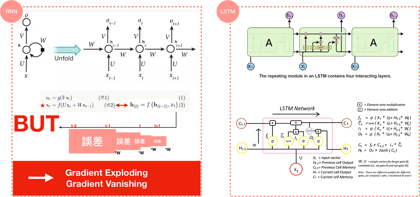
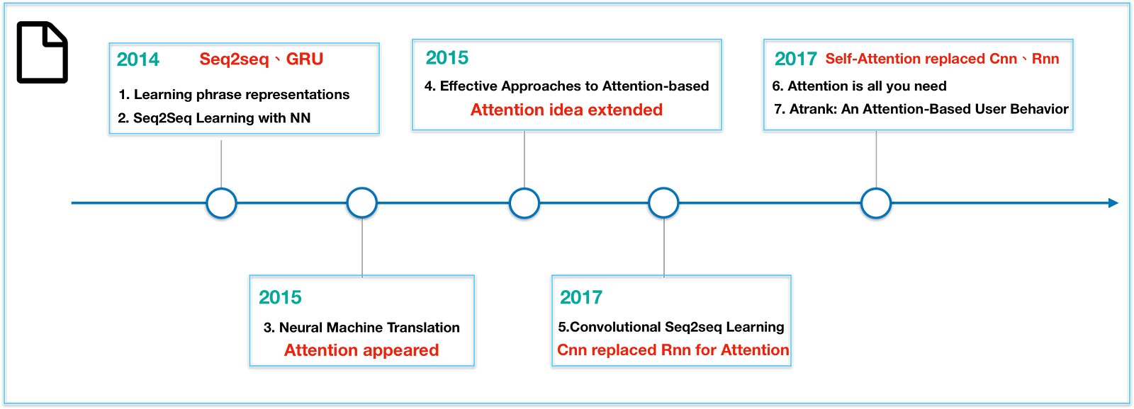
To prevent the weakness of RNN, LSTM came up as a savior with some methods such as forget/input/output gate, cell memory, hidden state, etc. In 2014, paper Learning Phrase Representations also propose a new model called GRU, which is much simpler to compute and implement. LSTM, GRU are two particular type of recurrent neural networks that got lots of attention within the deep learning community.

These are some applications of LSTM models in Figure(5). However, we will not dive into them in this article.

Seq2seq

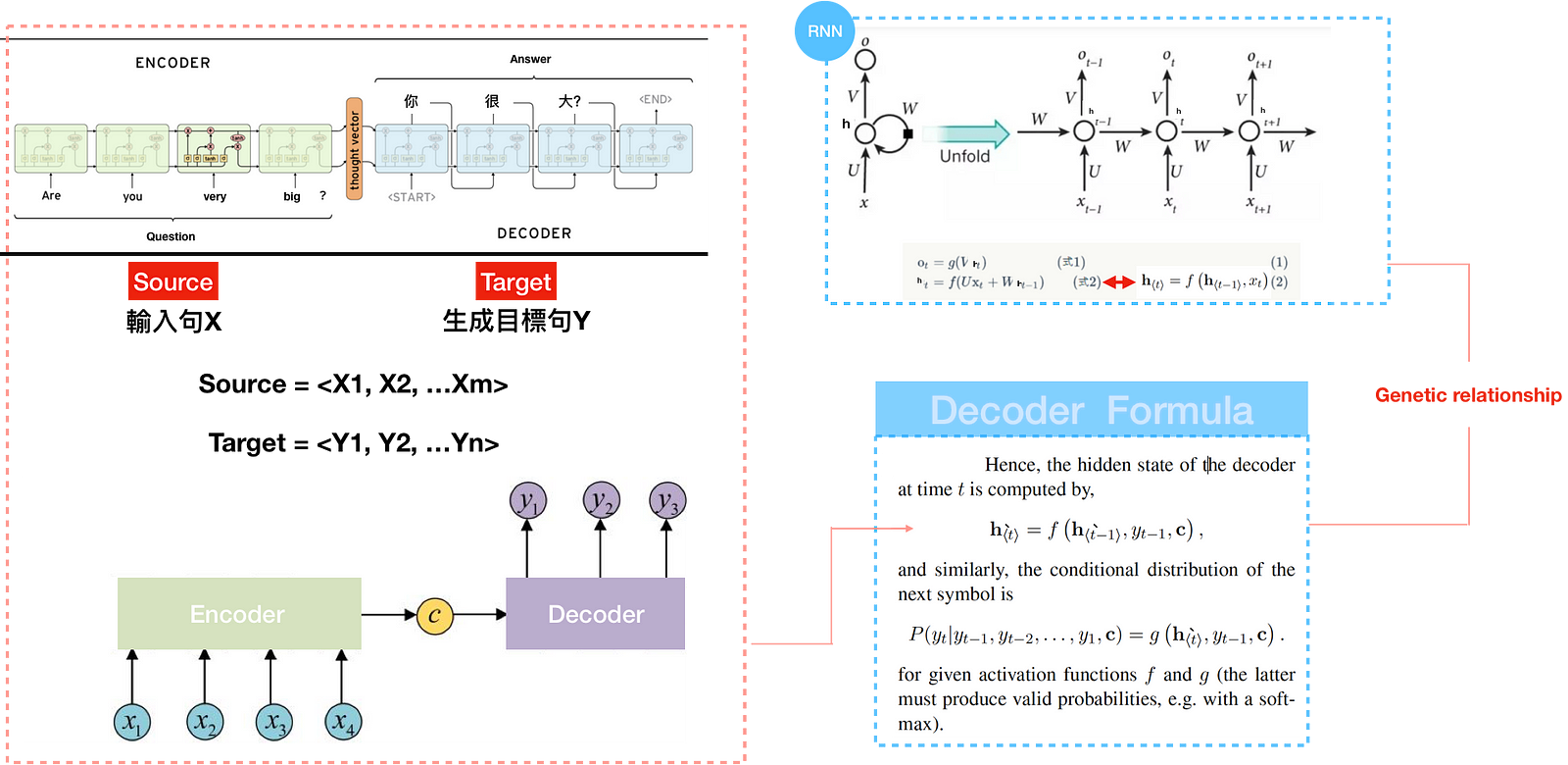
Back to the topic. In Figure(6), It’s obvious that Seq2seq model consists of Encoder and Decoder. Once inputing source sentence into the encoder, you will get the target sentence from the decoder. With the preliminary knowledge of RNN, you can find the formula of Seq2seq is similar to RNN, but with a new item called context vector. Context vector is also known as thought vector with sentence embedding information inside, which is the final hidden state of the encoder. An encoder processes the input sequence and compresses the information into a context vector of a fixed length. This representation is expected to be a good summary of the meaning of the whole source sentence. The decoder is then initialized with the context vector to generate output — figure(7).

However, In seq2seq model, source information is compressed in a fixed-length context vector. A critical disadvantage of this design is incapability of long sentences memory and leads to bad result.

In 2015, the attention model was born to resolve this problem.

Attention model

Why attention model?

The attention model was born to help memorize long source sentences in neural machine translation.

Instead of building a single context vector out of the encoder’s last hidden state, this new architecture create context vector for each input word. For example, If a source sentence has N input word, then there’s get to be with N context vectors rather than one. The advantage is that the encoded information will be much great decoded by the model.

Here, the Encoder generates <h1,h2,h….hm> from the source sentence <X1,X2,X3…Xm>. So far, the architecture remains the same as the Seq2seq model. Source sentence as input and Target sentence as output. Therefore, we want to figure out the difference inside the model, which is the context vector c_{i} for each of the input word in Figure(10).

The question is how to calculate the context vector c_{i}.

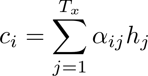
Context vector c_{i} is a sum of hidden states of the input sequence, weighted by attention scores α — equation(1). Attention/Alignment score is the most important idea in attention model for interpreting word importance. Since attention score is calculated by score e_{ij}, let’s talked about score e_{ij} first.

a is an Alignment model that assigns a score e_{i,j} to the pair of input at position j and output at position i, based on how well they fit. e_{i,j} are weights defining how much of RNN decoder hidden state s_{i-1} and the j-th annotation h_{j} of the source sentence should be considered for each output — equation(3).

score e_{ij}, later has been interpreted as part of global attention and soft attention in the paper Effective approaches of the NMT and Show, Attend and Tell. We can transform the score e_{ij} into score(h_{t}, \bar {h_{s}}), where h_{t} maps s_{i-1} and \bar {h_{s}} maps h_{j} from above — Figure(11). As you can see, there are many ways for calculating the score. We can simply take dot for easy use.

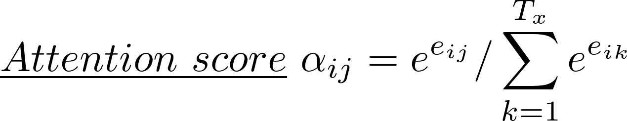
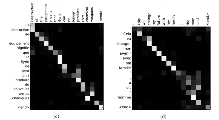
Once you have the score e_{ij}, the attention score α is then parametrized by a feed-forward network , alignment model a, calculated with softmax — equation(2) and context vector is done. This network is jointly trained with other parts of the model. With the matrix of attention scores, it is nice to see the correlation between source and target words.

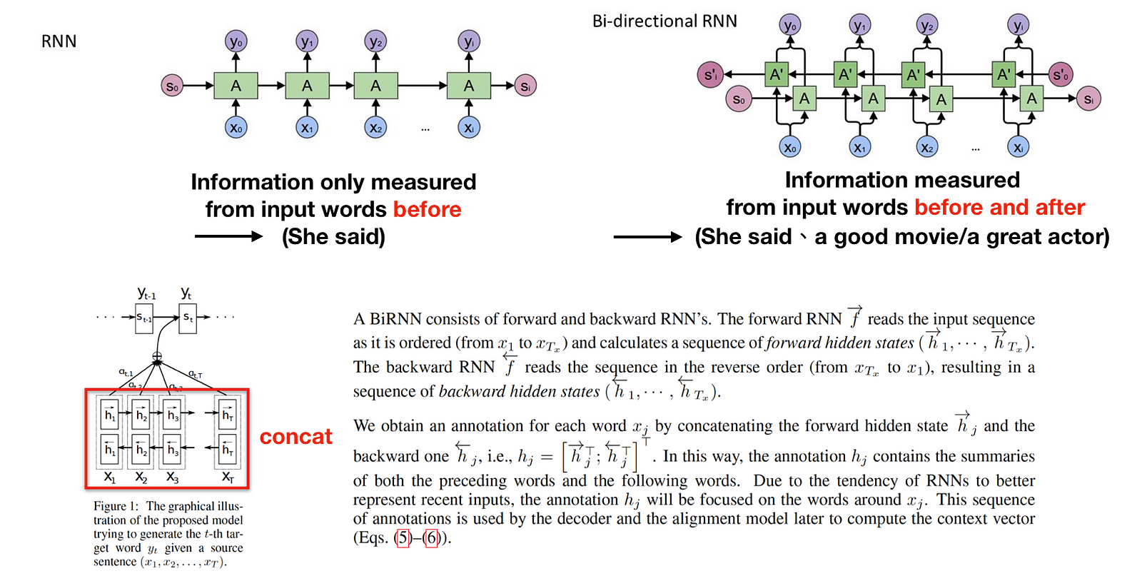
Finally, the encoder uses Bi-directional RNN for better understandings of the context from future time steps. Take the following examples, “She said, The rock is a good movie” and “She said, The rock is a great actor”. In the above two sentences, when we are looking at the word “The rock” and the previous two words “She said”, we might not be able to understand if the sentence refers to the movie or actor. Therefore, we need to look ahead to resolve this ambiguity. This is how Bidirectional RNN works.

However, Attenion model still faces some problems. One disadvantage is that the context vector is calucated through hidden state between source and target sentence, leaving the attention inside source sentence and target sentence itself ignored — see Figure(11). Another is that RNN is hard to parallelize, leading the calculation time-consuming. Some paper trying to resolve the problem through CNN model. In fact, CNN model uses lots of layers to minimize the weakness of local information. Because of these shortcomings, Google introduced self attention to resolve them in 2017.

Let’s recap a classic Seq2seq model & Attention-based model in Fig.15. The difference between them is the calculation of context vector.

Conclusion

So far, we have a a brief overview of the Seq2seq model and Attention-based model. I strongly recommend you to read those classic paper for a deeper understanding.

In the next part, I will be focusing on self attention, proposed by Google in the paper “Attention is all you need”. The model proposed by this paper abandoned the architecture of RNN and CNN.