We have talked about Seq2seq and Attention model in the first part. In this part, I will be focusing on Self attention, proposed by Google in the paper “Attention is all you need”. Self attention is the concept of “The transformer”model, which outperforms the attention model in various tasks. Two main concepts of the “transformer” model are “self attention” and “multi-head”.

The biggest advantage comes from how The Transformer lends itself to parallelization and self attention.

Hope you enjoy it.

Preface

I will use the figure in part 1 as a quick overview. We now know how attention model works. The disadvantage of attention model is that it cannot be parallelize and ignore the attention information inside source sentence and target sentence. In 2017, Self Attention was born to resolve this problem.

Self Attention

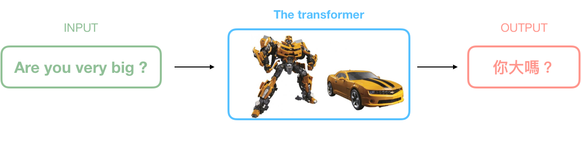
Self attention is proposed in the paper “Attention is all you need”, which is the core concept of the model “The transformer”. We can think of the “The transformer” as a black box. Once sending source sentence inside, we will get the output sentence.

Especially, “The transformer” abandoned the architecture of RNN and CNN.

The transformer

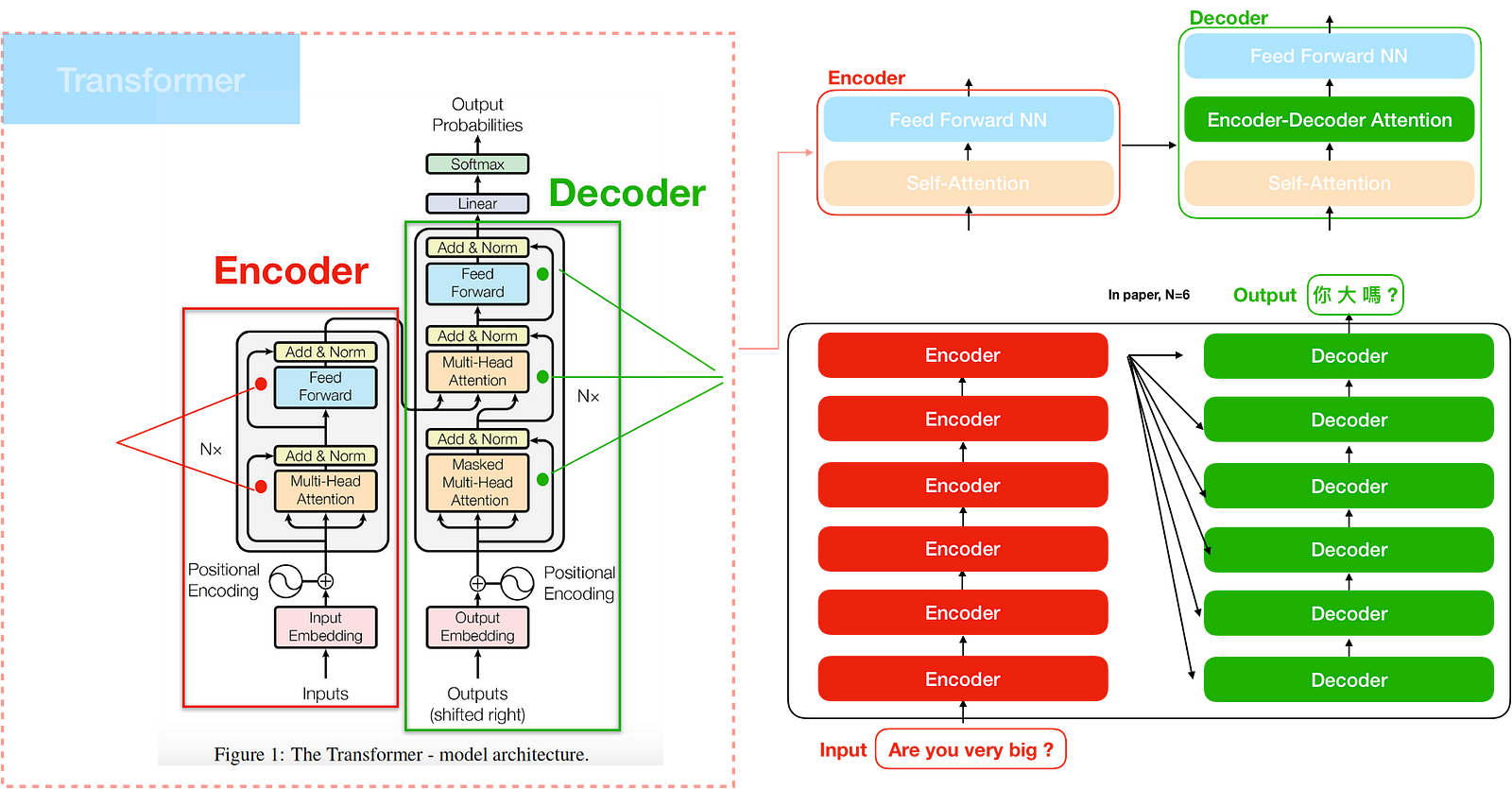
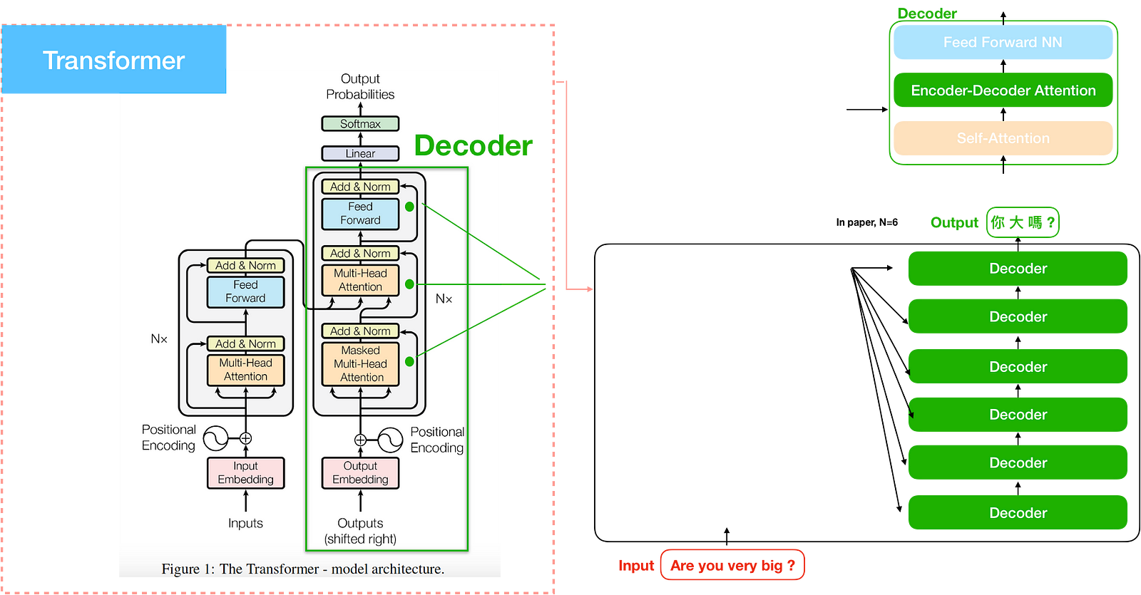
The transformer consists of two parts. Just as usual, one is the encoder and the other is the decoder. However, The encoder is a stack of encoders (the paper stacks six of them on top of each other). The decoder is a stack of decoders of the same number. These mechanisms are different with attention model.

Query, Key, Value

Before we dive into the transformer, some concepts of attention model should be renewed. In attention model, the Encoder generates <h1,h2,h….hm> from the source sentence <X1,X2,X3…Xm>. Context vector c_{i} is a sum of hidden states of the input sequence, weighted by attention scores α. With context vector and hidden state, we can then calculate output sentence<y1…yn>.

Let’s translate that in another words.

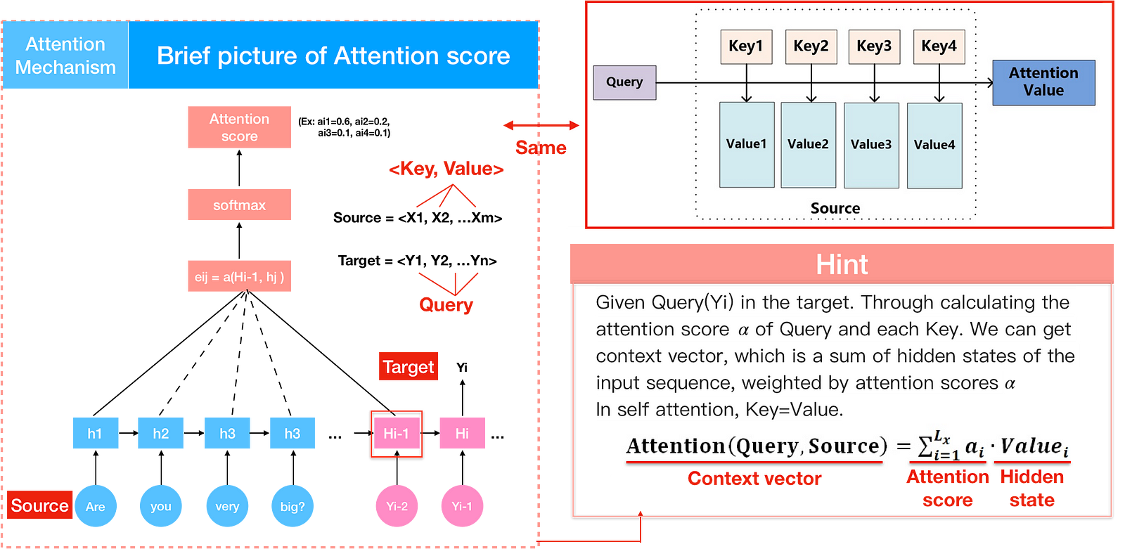
Input word in source sentence are pairs of <(Address)Key, (element)Value> and output word in target sentence is Query — Figure(4 left). We can then turn the calculation of context vector into another interpretation by Key, Query and Value — Figure(4 right). Through the calculation of similarity between Query and each Key, we can get the attention score of the Value, corresponding to the Key. Attention score is the importance of a input word. We then multiply each value vector by the attention score and sum up the weighted value vector, which is Attention/context vector.

In my opinion, this is the hardest part when reading paper from attention model to self attention for this renewal translation not being explained in the paper. You can also read the paper Key-Value Memory Networks for Directly Reading Documents, where the idea of key and value appeared.

We can now reinterpret the decoder formula in attention model. Calculating attention vector comes mainly in three steps. First, we take the query and each key and compute the similarity between the two to obtain a score e_{ij}. We have met 3 kinds of similarity functions in part 1 figure(11), though we used dot in the end. The second step is to get attention score a_{i} by using a softmax function to normalize these scores, and finally to weight these weights in conjunction with the corresponding values and obtain the attention/context vector, c_{i}.

In current NLP work, the key and value are usually came to the same thing, therefore key=value.

Now we have the concept of Query, Key and Value, we can go through “the transformer”.

Scaled Dot-Product Attention

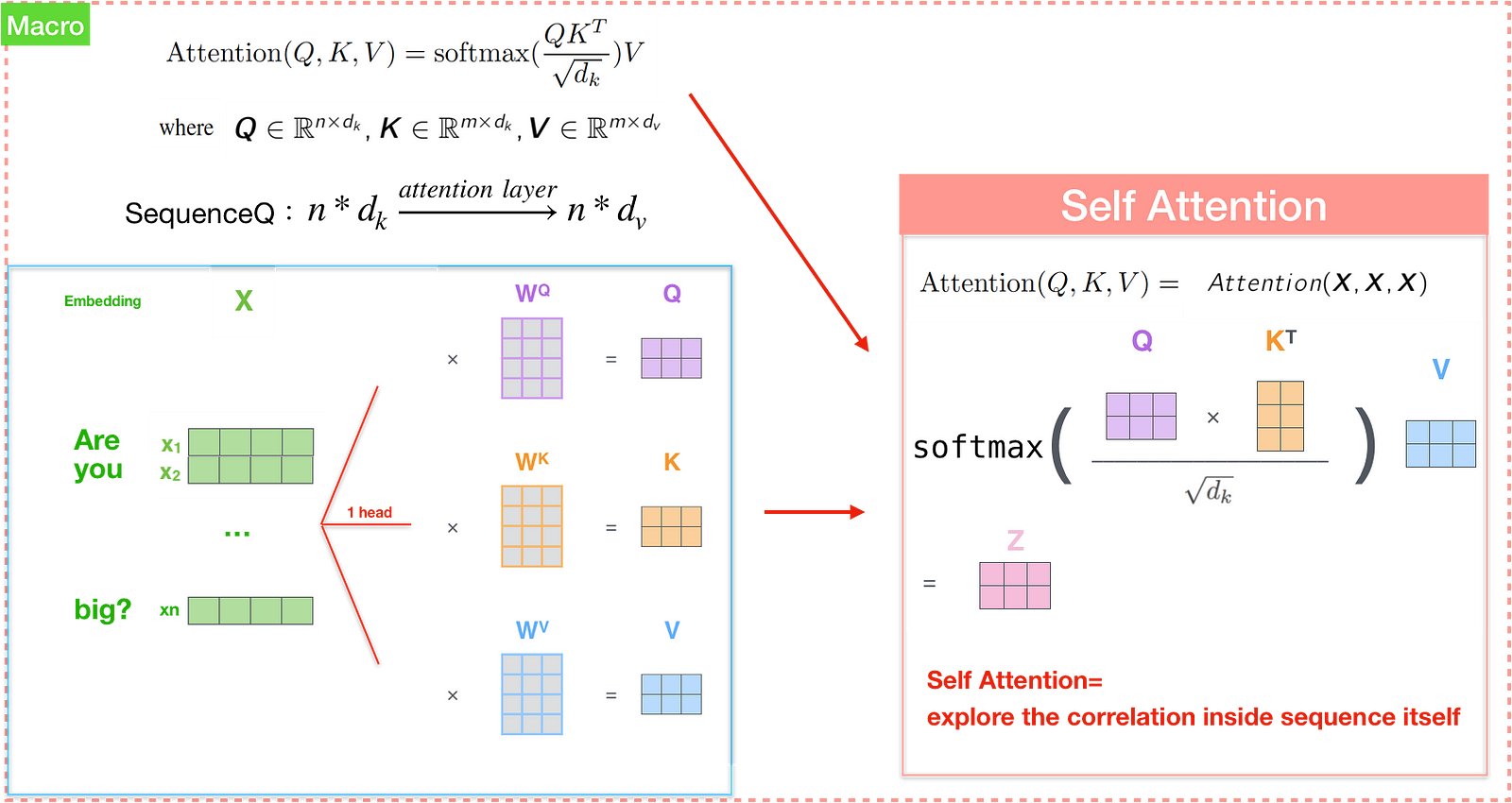
The transformer uses a particular form of attention called the “Scaled Dot-Product Attention” which is computed according to the following equation in figure(6). Compared to the standard form of attention described in the attention model, Scaled Dot-Product Attention is a type of attention that utilizes Scaled Dot-Product with division \sqrt_{d_{k}}to calculate similarity. We can find that the attention idea remains the same with attention model, but differs in the addition of division \sqrt_{d_{k}}. The difference is that it has a division \sqrt_{d_{k}} for adjustment that prevents the inner product from becoming too large — figure(6). Also, Attention(q_{t}, K,V) are the same as calculated in attention model from a microcosmic perspective.

In other words, The transformer model is similar to attention model, except for their description of terms.

Three kinds of Attention

The transformer contains three main attention. One is the encoder self attention in encoder. Another is the decoder self attention in decoder. The other is the encoder-decoder attention, which is similar to the concept of attention model. Let’s start with encoder/decoder self attention from their corresponding encoder/decoder.

Encoder

The encoder is the left part of the transformer model. In this paper, the encoder is a stack of encoders (the paper stacks six of them on top of each other). Inside the encoder is multi-head encoder self attention. We will talk about multi-head later.

How to calculate encoder self attention?

We will take a look from the microcosmic perspective by vectors Attention(q_{t}, K, V), then proceed to look at how it’s actually implemented with matrices.

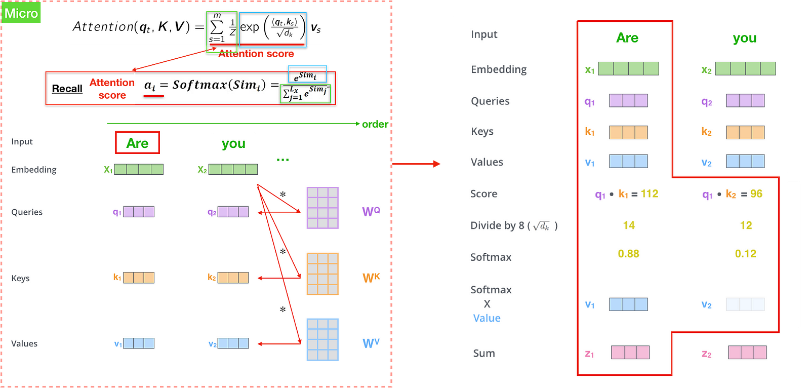
The first step in calculating self-attention is to create three vectors from each of the encoder’s input vectors (in this case, the embedding of each word in “Are you very big?”). Then we multiply the embeddings by three different matrices to create a Query vector, a Key vector, and a Value vector for each word. In this paper, outputs of dimension d_{model}=512.

The second step in calculating self-attention is to calculate a score <q_{t}, k_{s}> by taking the dot product of the query vector with the key vector of the respective word we’re scoring, which is similar to e_{ij} in attention model. Say we’re calculating the self-attention for the first word in this example, “Are”. We need to score each word of the input sentence such as “you”, ‘very’, ‘big?’ against this word. The score determines how much focus to place on other parts of the input sentence as we encode a word at a certain position. So if we’re processing the self-attention for the word in position #1, the first score would be the dot product of q1 and k1 (“Are vs Are”). The second score would be the dot product of q1 and k2(“Are vs you”).

The third step is to divide the scores by \sqrt_{d_{k}} (the paper assumes d_{k} = 64.), then pass the result into exponential with division 1/Z. The result is attention/softmax score. Interestingly, we can turn this structure into softmax description where Z equals the sum of exponential — Figure(9). This attention score determines how much each word will be expressed at this position, just like how attention model did. Clearly the word at this position will have the highest softmax score, but sometimes it’s useful to attend to another word that is relevant to the current word.

The final step is to multiply each value vector by the attention score, then sum up the weighted value vectors (z_{i}). This produces the output of the self-attention layer at this position (for the first word), similar to context vector in attention model — figure(9).

That concludes the self-attention calculation. The resulting vector is the one we can send along to the feed-forward neural network. In the actual implementation, this calculation is done in matrix form — figure(10).

Multi-head attention

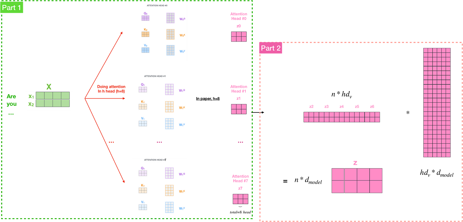
If we only computed a single attention weighted sum of the values, it would be hard to capture diverse representations of the input. To improve the performance of the model, instead of doing a single attention function with d_{model}-dimensional keys, values and queries, authors found it beneficial to linearly project the queries, keys and values h times with different linear projections to d_{q}, d_{k} and d_{v} dimensions, respectively. In the paper, d_{k}=d_{v}=d_{model}/h=64.

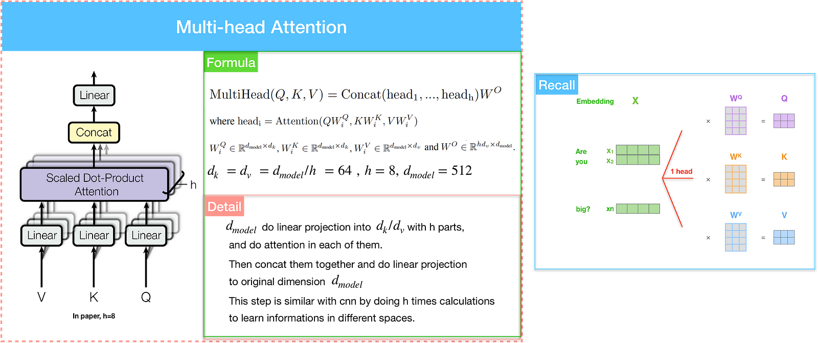
Also, the Transformer uses eight attention heads, so we end up with eight sets for each encoder/decoder. Each set is used to project the input embeddings into a different representation subspace. If we do the same self-attention calculation we described before, we end up with eight different Z matrices. However, the feed-forward layer is not expecting eight matrices. We need to concatenate them and condense these eight down into a single matrix by multiply them with an additional weights matrix WO — figure(12).

Residual Connections

One detail in the architecture of the encoder that we need to mention before moving on, is that each sub-layer (self-attention, feed-forward networks) in each encoder has a residual connection followed by a layer-normalization.

A residual connection is basically just taking the input and adding it to the output of the sub-network, making training deep networks easier in the field of computer vision. Layer normalization is a normalization method in deep learning that is similar to batch normalization. In layer normalization, the statistics are computed across each feature and are independent of other examples. The independence between inputs means that each input has a different normalization operation.

Position-wise Feed-Forward Networks

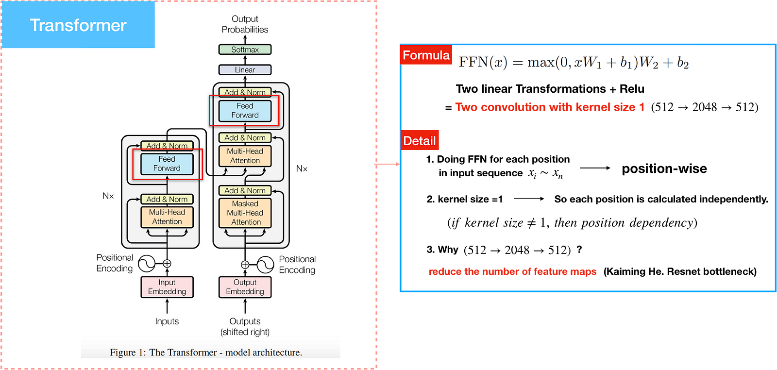
In encoder and decoder the attention sublayers is being processed by a fully connected FFN. It is applied to each position separately and identically meaning two linear transformations and a ReLU. For example, if input sequence = <x1,x2…xm>, total size of position are m .

Linear transformations are the same for each position, but use different parameters from layer to layer. It works similarly to two convolutions of kernel size 1. It is only when kernel size=1 that remains position dependency, similar to CNN. The input/output dimension is d_{model}=512 while the dimension of inner layer is 2048. The idea, proposed by the genius Kaiming He.), is that it reduce the of feature maps when having calculation.

Positional Encoding

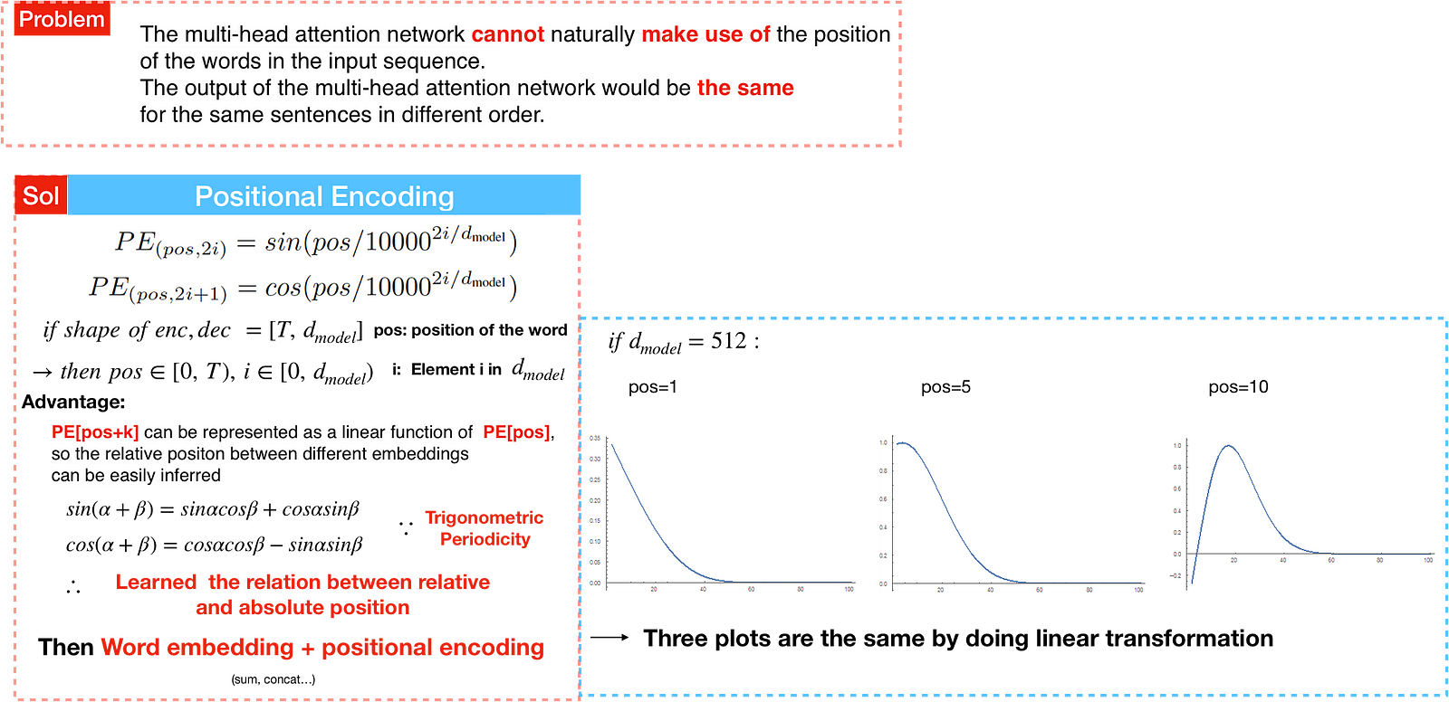
Unlike recurrent networks, the multi-head attention network cannot naturally make use of the position of the words in the input sequence. Without positional encodings, the output of the multi-head attention network would be the same for the same sentences in different order. For example, “Are you very big?” and “Are big very you?”. Positional encodings explicitly encode the relative/absolute positions of the inputs as vectors and are then added to the input embeddings.

The paper uses the equation PE(pos, 2i)=sin(pos/10000^{2i/d_{model}}) to compute the positional encodings, where pos represents the position, and i is the dimension. Basically, each dimension of the positional encoding is a wave with a different frequency. This allows the model to easily learn to attend to relative positions, since PE[pos+k] can be represented as a linear function of PE[pos], so the relative positon between different embeddings can be easily inferred.

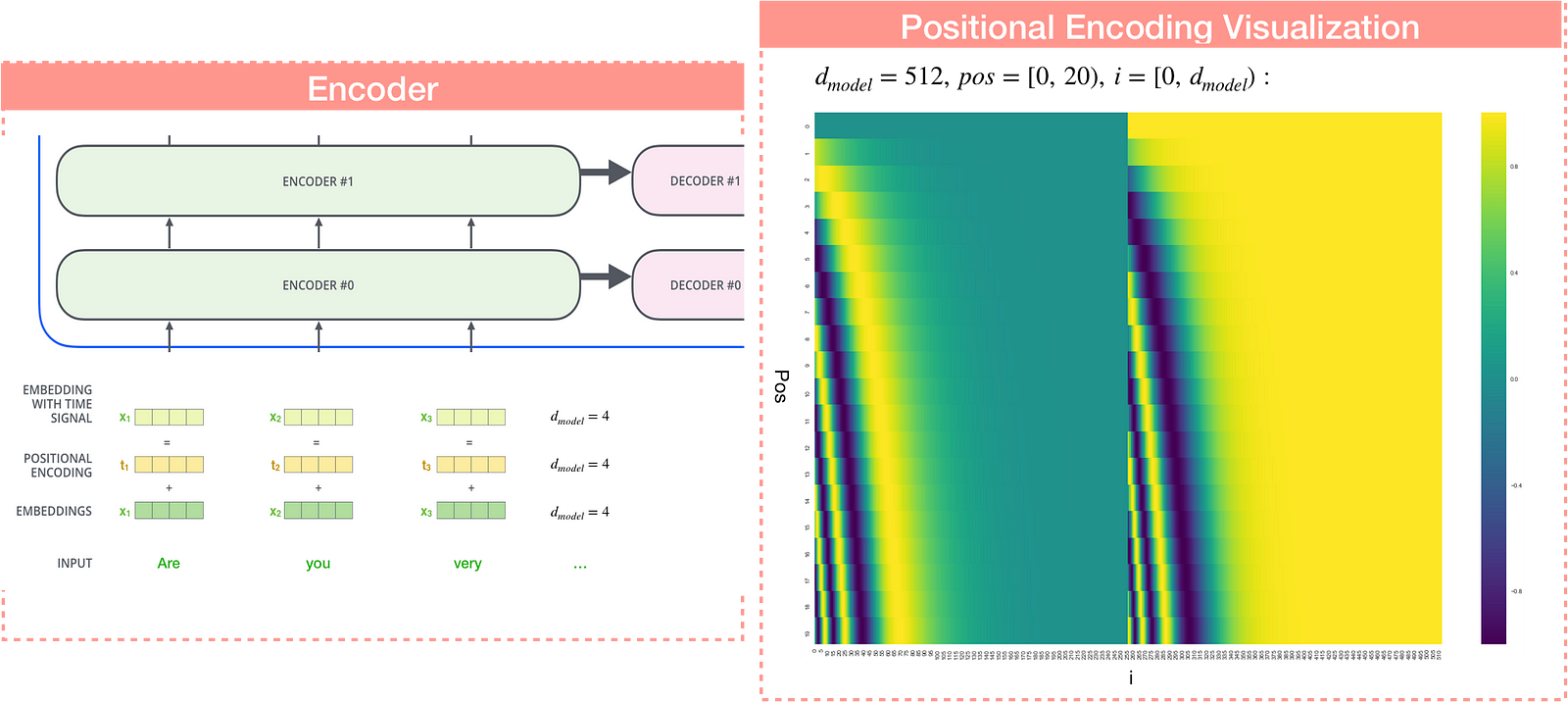
If we assumed the embedding has a dimensionality of 4, the actual positional encodings would look like this:

In the following figure, each row corresponds the a positional encoding of a vector. So the first row would be the vector we’d add to the embedding of the first word in an input sequence. Each row contains d_{model} values with pos rows, which is the count of input word in a sentece. For example, source sentence has 20 word with each word embedding=512. We’ve colored them so the pattern is visible.

Now that we’ve covered most of the concepts on the encoder side, let’s take a look at how decoder works.

Decoder

Masked multi-head attention

Similar to the encoder, residual connections are employed around each of the sub-layers, followed by layer normalization.

In encoder, self-attention layers process input queries,keys and values that comes from same place i.e. the output of previous layer in encoder. Each position in encoder can attend to all positions from previous layer of the encoder. In decoder, self-attention layer enable each position to attend to all previous positions in the decoder, including the current position.

However, to prevent positions from attending to subsequent position. In other words, the self-attention layer is only allowed to attend to earlier positions in the output sequence. Masking multi-head attention is done by masking future positions (setting them to -∞) before the softmax step in the self-attention calculation. This step ensures that the predictions for position i can depend only on the known outputs at positions less than i.

Encoder-Decoder Attention

The “Encoder-Decoder Attention” layer is different with Encoder/Decoder attention layer. Unlike multi-head self-attention, Encoder-Decoder Attention creates its Queries matrix from the layer below it, which is decoder self attention, and takes the Keys and Values matrix from the output of the encoder stack.

Now that we’ve covered most of the concepts on the encoder/decoder side, Let’s take a look at how they work together.

The encoder start by processing the input sequence. The output of the top encoder is then transformed into a set of attention vectors K and V. These are to be used by each decoder in its “encoder-decoder attention” layer which helps the decoder focus on appropriate places in the input sequence.

The Final Linear and Softmax Layer

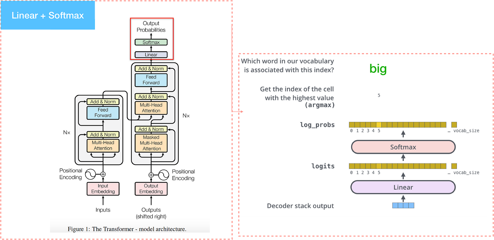
The decoder stack outputs a vector and passes into the final Linear layer which is followed by a Softmax Layer.

The Linear layer is a simple fully connected neural network that projects the vector produced by the stack of decoders, into a logits vector with score of a unique word. The softmax layer then turns those scores into probabilities. The highest probability is chosen as the word output for this time step.

Why self attention?

Traditionally, both the encoder and the decoder were composed of recurrent neural networks (RNNs). RNNs sequentially process the input sequence (x1…, xn) into hidden encodings (h1…hn), then sequentially generate the output sequence (y1…yn). However, the sequential nature of RNN means it is impossible to compute in parallel. Also, the total computational complexity per layer is enormous. Most important, learning long-range dependencies in the network is difficult.

Through “the transformer”, we can resolve the parallellization and computational complexity by multi-head attention. The problem of long-range dependencies is also improved through self attention with 1-length in each word.

Future

In financial industry, it’s fruitful to portrait a customer through customer journey so that we can have a better understanding of how consumers interact and engage with our brand. However, it’s hard to extract information from customer journey without any feature engineering. Especially “journey” is a sequence behavior rather than a specific feature. With the knowledge of self-attention, we can further implement the concecpt and create value from complex data in our company.

It is recommended to read the paper ATrank published by Alibaba. Alibaba used the framework of self attention for product recommendation and achieved better performance.

Reference

[1] Learning Phrase Representations using RNN Encoder–Decoder for Statistical Machine Translationr. arXiv:1406.1078v3 (2014).

[2] Sequence to Sequence Learning with Neural Networks. arXiv:1409.3215v3 (2014).

[3] Neural machine translation by joint learning to align and translate. arXiv:1409.0473v7 (2016).

[4] Effective Approaches to Attention-based Neural Machine Translation. arXiv:1508.0402v5 (2015).

[5] Convolutional Sequence to Sequence learning. arXiv:1705.03122v3(2017).

[6] Attention Is All You Need. arXiv:1706.03762v5 (2017).

[7] ATRank: An Attention-Based User Behavior Modeling Framework for Recommendation. arXiv:1711.06632v2 (2017).

[8] Key-Value Memory Networks for Directly Reading Documents. arXiv:1606.03126v2 (2016).

[9] Show, Attend and Tell: Neural Image Caption Generation with Visual Attention. arXiv:1502.03044v3 (2016).

[10] Deep Residual Learning for Image Recognition. arXiv:1512.03385v1 (2015).

[11] Layer Normalization. arXiv:1607.06450v1 (2016).