The Intuition Behind Artificial Neural Networks

Explaining ANNs by analogy to the human brain

The Neuron

Brains are the best weapons of learning and they are built from neural networks. This is a network or neutrons, so how do neutrons actually work?

Body, dendrites (receiver) and axon (transmitter). Messages are sent which stimulate the receiver’s dendrites. This reception area is called the synapse.

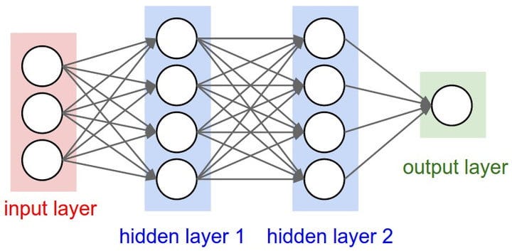
So how do we create a neutron in a machine? Consider a neutron as a node with several input values and one output signal. The input values may also be neutrons (hidden layers). These input values constitute the input layer (if it’s composed of other neutrons, it’s a hidden input layer).

The input layer is a bit like a collection of senses. Note that the brain is encased in a hard bone skull, a black box, and relies on these senses to collect information about the surroundings.

The connections between the input values and the node are equivalent to synapses.

Input layer:

• The independent variables are all from a single observation and should be standardised (mean 0, s.v. 1) or normalised (in the range 0–1) so that the input nodes have similar value ranges (helps efficiency).

Output values:

• Continuous (price)
• Binary (yes/no)
• Categorical variable (actually sever probabilities — one for each category)

Whichever one type of output is produced, it relates to a single observation’s input.

Each synapse gets assigned a weight which is crucial to the NN. These are how the NN learns: by adjusting the weights using tools like gradient descent and back propagation.

So What Happens Inside the Neuron?

Firstly, all of the input values get added together, according to their weights (simply multiply by the weight and sum). The activation function is applied to this weighted sum to determine the output value.

The Activation FunctionOptions:

• Threshold function: This is 0 or 1 depending if the weighted sum is bigger than the threshold
• Sidmoid function: This is smooth and continuous like a smooth threshold function. Values in the range (0,1) so better for predicting probability
• Rectifier function: This is 0 when the sum < 0 and uniformly increasing thereafter. Softplus is an alternative which is smooth.
• Hyperbolic tangent: Similar to the sigmoid function but in the range (-1,1)

Of course, a neural network is made up of a whole network of nodes arranged in (hidden) layers, and each node contains its own activation function.

How Do Neural Networks Work

Let’s take an example where we want to predict property prices, and let’s assume that we have a NN that is already trained up using the following input parameters: — Area — Bedrooms — Distance to the city — Age These parameters comprise the input layer. The output layer is the predicted price. In a simple case, these inputs would be weighted and summed to give a single output value.

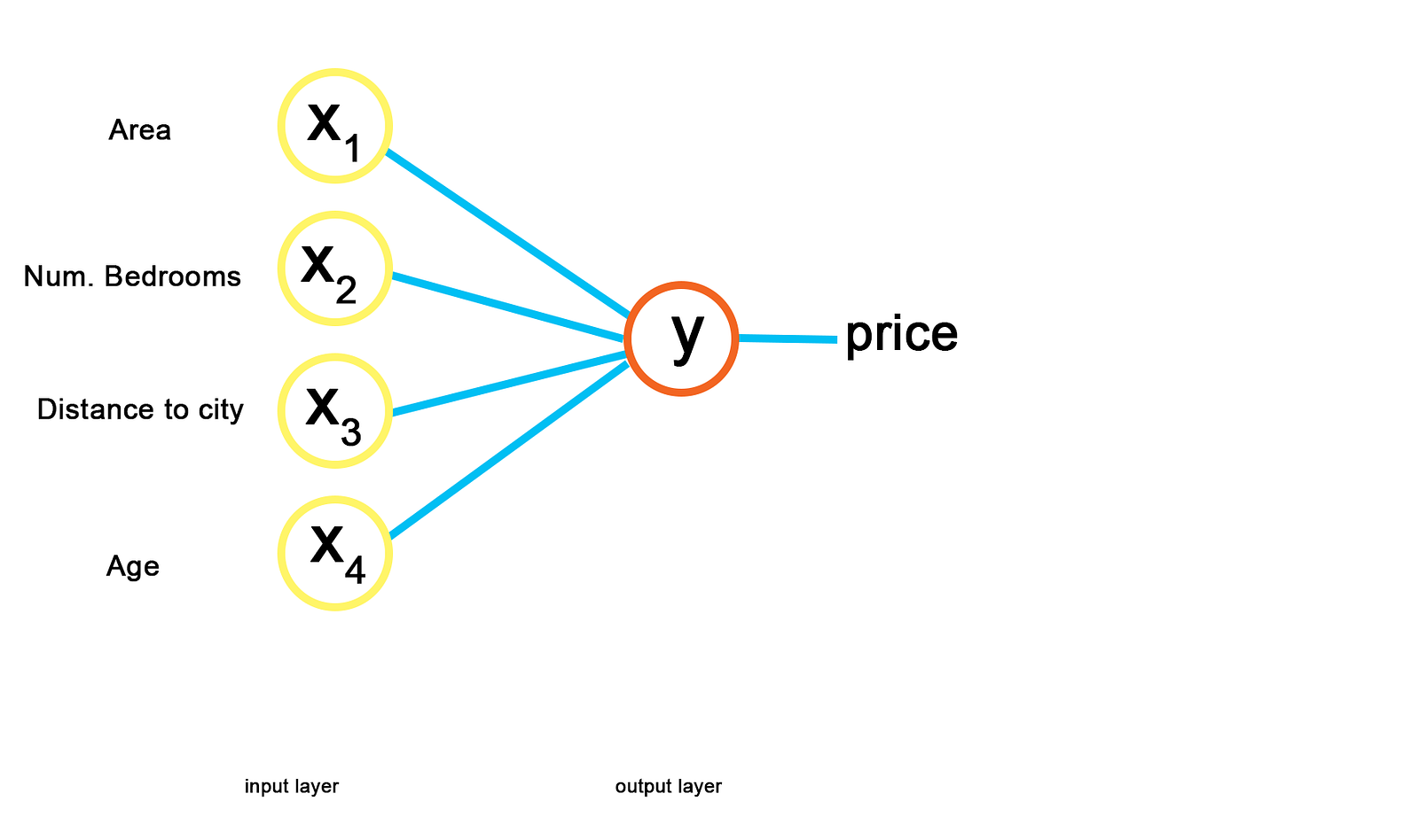
This is a very trivial representation of the problem and you can see it may be very inflexible, as well as sensitive to the input data.

This is where the hidden layers in an ANN become very important. Neurons in the hidden layer can react to different features of the input data and ignore others, simply by adjusting the weights.

Given a case with exactly one hidden layer, we can connect each input value in the input layer to each node of the hidden layer and weight their connections. Now, some weights may be zero because they may not be important to the neuron that they are connected to.

In the example, area and distance to the city may be correlated, but the number of bedrooms may not be correlated to these. The neuron then has the weight for number of bedrooms set to 0. Similarly, area, number of bedrooms and age may be correlated but distance may not be correlated with these, affecting the weights to the next neuron.

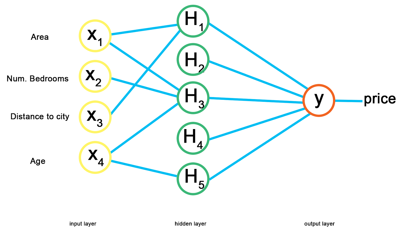
Try to work out a possible rationale for neuron H5.

Individually, each neuron cannot predict the price output, but in combination they become very powerful.

How Do Neural Networks Learn

Now, heres the important bit…

When programming the solution to a classification problem (for example) there are two options:

• hard-coded — this is based on rules and all actions and features are taken care of explicitly and programmed accordingly;
• alternatively, as in ANNs, provide a means to figure out how to convert inputs to outputs.

The goal of machine learning is to create a method (in the case of ANNs, this is a network) that learns on its own without deterministic rules. For a Neural Network, the idea is that it will learn and adjust the weights by itself.

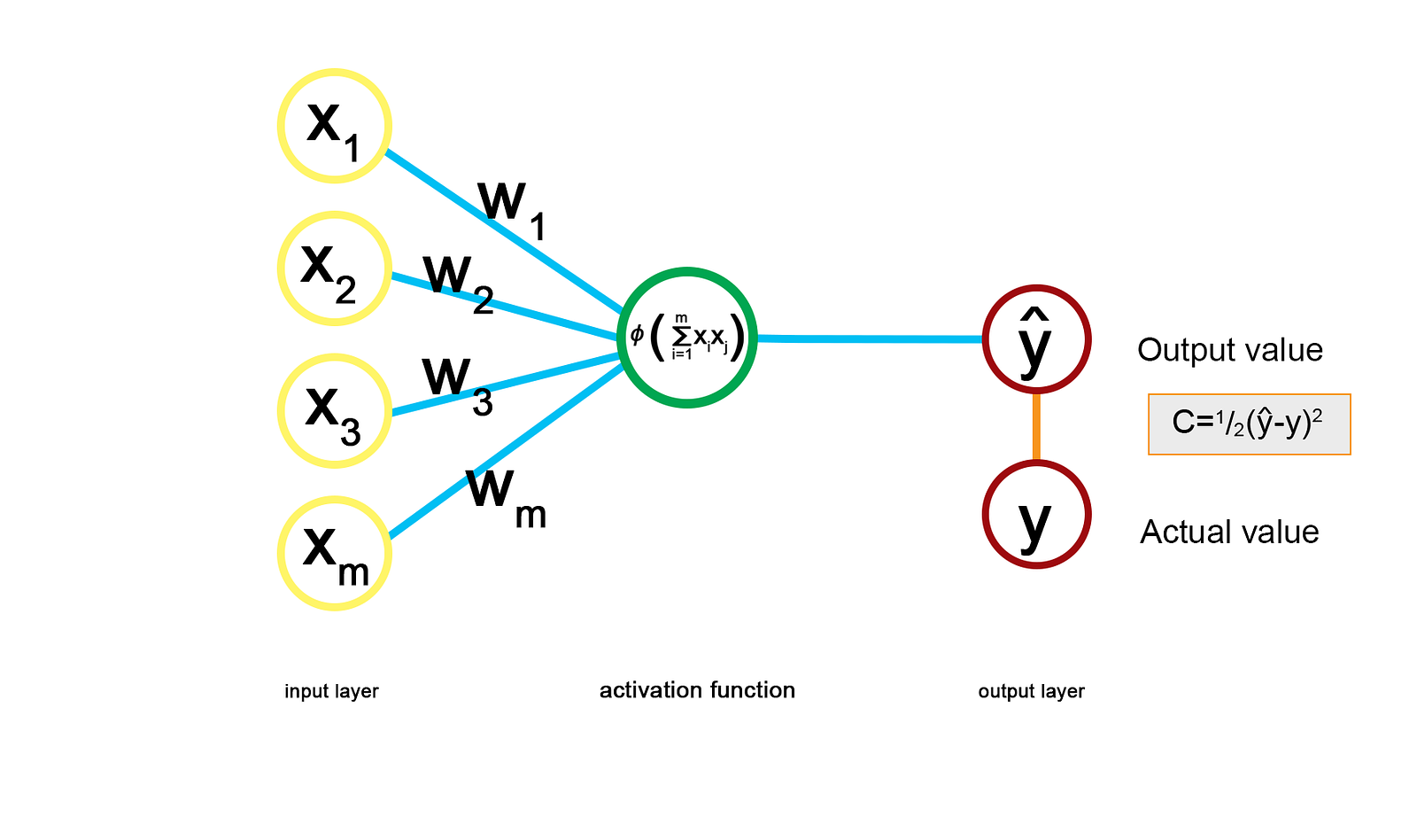
Notation: y^ is the value predicted by the ANN, and y is the actual value.

Then, for each input data-point, each value gets supplied to the perceptron and the activation function is applied. This produces the output value y^.

The next step is to compare the actual and output values and then calculate the value of the cost function. One of the most common cost functions is to calculate half of the squared distance between the two values, as shown above. The cost function shows the error in the prediction so we want to minimise this.

The result of the cost function is fed backwards through the perceptron and the weights are updated. The method for this is discussed later in this article.

So far we have only worked on one single data point with several features. If our dataset is made up of only a single point, we keep iteratively feeding in this datapoint and updating the weights until the cost function is below some threshold.

Now, supposing we have a whole dataset, we go through the whole dataset on each iteration, instead of just one data point. This is termed an ‘epoch’. After we obtain the output value for each input point, we compare to the actual values. The cost function for the whole dataset is the sum of the cost functions for each data point. We then update the weights and run further epochs until the cost function is minimised.

This whole process is called back-propagation. (See also cross-validated back-propagation.)

Gradient Descent

So far: in order for an Artificial Neural Network to learn, back-propagation of the error through the network must occur and the weights must be adjusted. So how do we adjust the weights?

One way could be to try out a large range of weights and plot the error accordingly. This is simple and intuitive if there is only one weight needing to be optimised. However, there are as many dimensions as there are input values in the input layers. A brute force approach would require testing k^m weights (where m is the number of inputs and k is the number of weight options to test for each). This then becomes a very complex task which could take a very long time.

Gradient descent is a solution that means we don’t have to test every possible combination. The general idea is to:

• Pick an initial point
• Test the gradient at this point (perhaps by testing a neighbour)
• Pick the next point in the direction of that downward gradient
• Continue until the gradient is within some threshold of zero-gradient

Of course, there may be complications as well as means to optimise the method. Furthermore, the method works in multiple dimensions.

Stochastic Gradient Descent

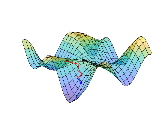
Gradient descent is a useful method, but requires a convex cost function (this is simple, with a single global minimum). If the cost function is not convex, then several minima may occur and the algorithm can get ‘stuck’ in one local minimum.

In GD, we look at all of the rows in the input data together. However, for stochastic GD, weight adjustment happens after each input, rather than after all of them. For both, there are multiple epochs. Stochastic GD helps to stop the minimisation from getting trapped into one local minimum. It causes the weights to fluctuate a lot more, but the result is that it has a greater chance of finding the global minimum than a local minima. It is also faster, as it requires less data to be used for each calculation.

See also the mini-batch gradient descent method.

Summary

1. Randomly initialise the weights to small numbers, close to 0.
2. Input the first observation in the input layer, where each feature in one input corresponds to one input node.
3. Forward propagation: from left-to right in our diagrams, the neutrons are activated such that the impact of each neurones activation is limited by the weights. These activations are propagated until the predicted result is obtained.
4. Compare the predicted and actual values.
5. Back Propagation: from right to left in our diagrams, update the weights according to how responsible they are for the calculated error. The learning rate decides by how much we update the the weights.
6. Repeat 1–5, updating the weights either:
7. After each observation — Reinforcement Learning
8. After a batch of observations — Batch Learning
9. Repeat for several epochs (where one epoch is completed when the whole training set has passed through the ANN).