Recently I started working on a speech classification problem, as I know very little about speech/audio processing, I had to recap the very basics. In this post, I want to go over some of the things I learned. For this purpose, I want to work on the “speech MNIST” dataset, i.e, a set of recorded spoken digits.

You can find the dataset here.

The dataset contains the following:

• 3 speakers
• 1,500 recordings (50 of each digit per speaker)

As mentioned in the title, this is a classification problem, we get a recording and we need to predict the spoken digit in it.

I want to try different approaches to this problem and understand step by step what works better and why.

First, let’s understand what audio recording is exactly. I’ll use the excellent librosa library for it:

wav, sr = librosa.load(DATA_DIR + random_file)print 'sr:', srprint 'wav shape:', wav.shape

# OUTPUTsr: 22050wav shape: (9609,)

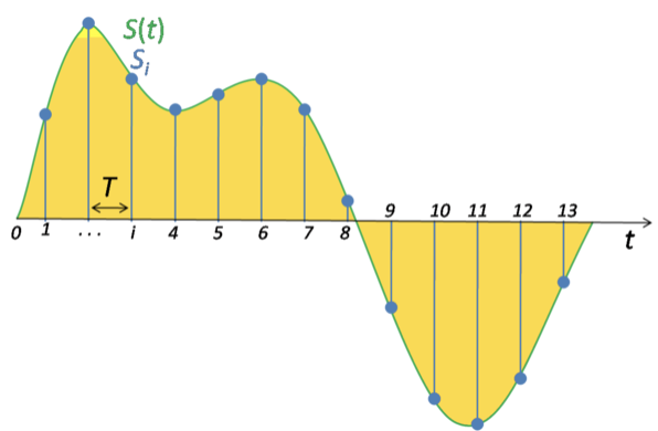
The load method returns 2 values, the first is the actual sound wave, and the second is the ‘sampling rate’. As you know, ‘sound’ is an analog signal, in order to make it digital and able to represent it with something like a numpy

array we have to sample the original signal. In short, sampling is simply “selecting” a finite number of points from the original signal and throw the rest. We can store these selected points in an array and perform different discrete operations on it. The Nyquist–Shannon sampling theorem showed that if our sampling rate is high enough, we are able to capture all the information in the signal and even fully recover it .

The sampling rate is very important, and we’ll use it later on in different algorithms. Its scale is Herz, i.e, number of points (samples) per second. In our example, sr=22050 so we have 22050 samples per second, and our wave size is 9609, we can calculate the audio length using this:

length = wav.shape[0]/float(sr) = 0.435 secs

Actually, our real sampling rate is not 22050, librosa implicitly re-sample our files to get the more standard 22050 SR. To get the original sampling rate we can use sr=False for the load method:

wav, sr = librosa.load(DATA_DIR + random_file, sr=None)print 'sr:', srprint 'wav shape:', wav.shapeprint 'length:', sr/wav.shape[0], 'secs'

# OUTPUTsr: 8000wav shape: (3486,)length: 0.43575 secs

The audio length remains the same as expected.

Resampling is useful when we deal with files with different sampling rates. We’ll stick with that for now.

The actual sound looks like this:

plt.plot(wav)

As you can see this is a very complex signal, it is very difficult to find patterns in it. Even if we zoom in, it is still quite complicated.

plt.plot(wav[4000:4200])

For a start, we’ll try to use these waves “as is” and try to build a neural network that will predict the spoken digit for us. In practice, it’s almost never done. I’m doing it here only to understand the different steps from raw file to a complete solution.

But first, we need to prepare our datasets. As we seen earlier, we have 1500 recordings of spoken digits by 3 speakers. Splitting the data into a classic 80–20 train test split might be not a good idea as our training data will contain the same speakers as in test data and probably will provide very good results while providing very bad results on other speakers. A proper way to test our algorithm is to train it on 2 speakers and test it on the third. This way we’ll have a very small training and test set, but for the purpose of this post, it is enough. In real life, we have to test our algorithms on many speakers with different genders, races, accents etc in order to truly understand how good our algorithm is.

Our data looks like this:

X = []y = []pad = lambda a, i: a[0: i] if a.shape[0] > i else np.hstack((a, np.zeros(i - a.shape[0])))for fname in os.listdir(DATA_DIR):    struct = fname.split('_')    digit = struct[0]    wav, sr = librosa.load(DATA_DIR + fname)    padded = pad(wav, 30000)    X.append(padded)    y.append(digit)

X = np.vstack(X)y = np.array(y)

print 'X:', X.shapeprint 'y:', y.shape

# OUTPUTX: (1500, 30000)y: (1500,)

We’ll use a simple MLP network with a single hidden layer for a start:

ip = Input(shape=(X[0].shape))hidden = Dense(128, activation='relu')(ip)op = Dense(10, activation='softmax')(hidden)model = Model(input=ip, output=op)

model.summary()

# OUTPUTLayer (type)                 Output Shape              Param #   =================================================================input_1 (InputLayer)         (None, 30000)             0         _________________________________________________________________dense_1 (Dense)              (None, 128)               3840128   _________________________________________________________________dense_2 (Dense)              (None, 10)                1290      =================================================================Total params: 3,841,418Trainable params: 3,841,418Non-trainable params: 0_________________________________________________________________

Let’s train it:

model.compile(loss='categorical_crossentropy',              optimizer='adam',              metrics=['accuracy'])

history = model.fit(train_X,          train_y,          epochs=10,          batch_size=32,          validation_data=(test_X, test_y))

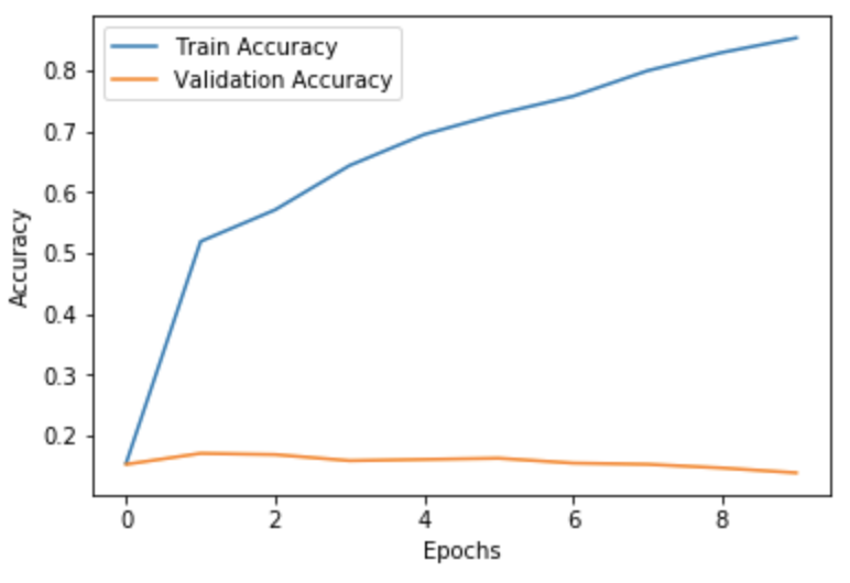
plt.plot(history.history['acc'], label='Train Accuracy')plt.plot(history.history['val_acc'], label='Validation Accuracy')plt.xlabel('Epochs')plt.ylabel('Accuracy')plt.legend()

You can see that our accuracy on the training data is somewhat ok, but it is horrible on our test data.

We can try different network architecture to maybe solve this issue, but as I said earlier, in practice, the raw waves almost never used. So we’ll move on to the more standard way to represent sound files: Spectrograms!

Before we talk about spectrograms, let’s talk about cosine waves.

A cosine wave looks like this:

signal = np.cos(np.arange(0, 20, 0.2))plt.plot(signal)

You can see that this is a pretty simple signal, there’s a clear pattern in it. We can control the cosine wave by changing the amplitude and the frequency of the wave.

signal = 2*np.cos(np.arange(0, 20, 0.2)*2)plt.plot(signal)

By adding together different cosine waves with different frequencies, we can achieve very complex waves.

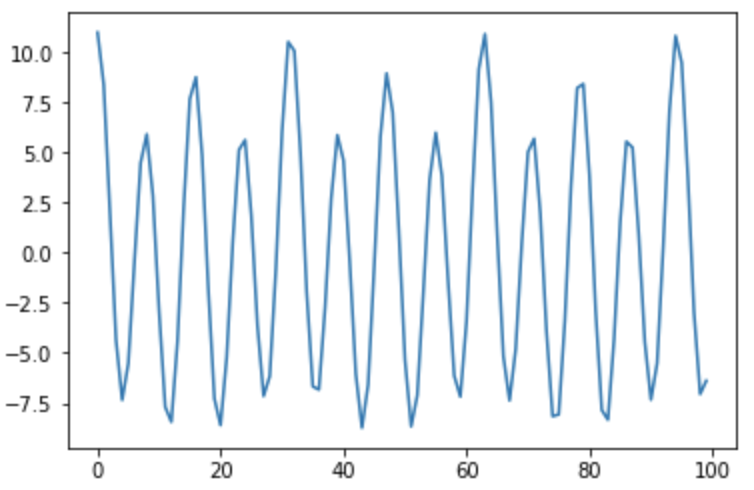
cos1 = np.cos(np.arange(0, 20, 0.2))cos2 = 2*np.cos(np.arange(0, 20, 0.2)*2)cos3 = 8*np.cos(np.arange(0, 20, 0.2)*4)signal = cos1 + cos2 + cos3plt.plot(signal)

We can represent the wave above in (at least) two ways. We can use the whole 100 size signal that is very complex, or, we can store only what frequencies were used in this signal. This is a much simpler representation of the data and with much less space used. Here we have 3 different frequencies with different amplitudes. What exactly are those 3 frequencies? this is a good question, and the answer is: it depends on the sampling rate (I will show later how).

We need a method that given a raw wave (a function of time), will return us the frequencies in it. This is what Fourier transform is for! I won’t dive into how Fourier Transform works, so let’s treat it as a black box that gives us the frequencies of a sound wave. If you want to understand it better, I recommend this video.

We need to decide what is the sampling rate of our wave, or, similarly, what is the length of our signal. Let’s use one second for convenience. We have 100 pints, so our sampling rate is 100 Hz.

Now we can use Fourier Transform for our signal. We’ll use the “Fast Fourier Transform” algorithm that calculates the Discrete Fourier Transform in O(nlogn). We’ll use numpy for that

fft = np.fft.fft(signal)[:50]fft = np.abs(fft)plt.plot(fft)

We see here 3 frequencies: 4, 7 and 14 bits per second, exactly as we built our signal (you’re welcome to check that).

Here we use only the first half of the return value because the result of FFT is symmetric.

It turns out that every sound (even human speech) is composed of many such basic cosine waves in different frequencies.

We have a way to get frequencies out of any sound signal, but human speech is not a static noise, it changes over time, So to correctly represent human speech, we’ll break our recordings into small windows and compute what frequencies are used in each window. We can use the Short-time Fourier transform for this.

D = librosa.amplitude_to_db(np.abs(librosa.stft(wav)), ref=np.max)librosa.display.specshow(D, y_axis='linear')

We can see some low frequency sounds in the middle of the recording. This is typical to a male voice. This exactly what a spectrogram is! It shows us different frequencies in different parts of the voice recording.

Let’s go over the code:

librosa.stft Computes the Short Time Fourier Transform for us. The return values is a matrix where X is the window numbers and Y are the frequencies. STFT values are complex numbers. We need use only the real part of it to find the frequency coefficients.

np.abs Takes the absolute of the stft in case of complex number it returns the absolute of the real part.

librosa.amplitude_to_db Converts the values to Decibels.

To recap:

Fourier Transform — The process of transforming a time-amplitude signal into a frequency-amplitude function

Discrete Fourier Transform (DST) — Fourier Transform discrete signal

Fast Fourier Transform (FFT)— An algorithm that is able to compute the Fourier Transform in O(nlogn) instead of O(n²)

Short-time Fourier transform (STFT) — Algorithm that breaks the recording into small windows and computes DST for each window

Great, now we are able to compute spectrograms for each file in our dataset and then use them to classify digits. What’s really nice about spectrograms is that they are like 2D images so we can use image classification techniques on them, specifically Convolutional Neural Networks!

ip = Input(shape=train_X_ex[0].shape)m = Conv2D(32, kernel_size=(4, 4), activation='relu', padding='same')(ip)m = MaxPooling2D(pool_size=(4, 4))(m)m = Dropout(0.2)(m)m = Conv2D(64, kernel_size=(4, 4), activation='relu')(ip)m = MaxPooling2D(pool_size=(4, 4))(m)m = Dropout(0.2)(m)m = Flatten()(m)m = Dense(32, activation='relu')(m)op = Dense(10, activation='softmax')(m)

model = Model(input=ip, output=op)

model.summary()

# OUTPUTLayer (type)                 Output Shape              Param #   =================================================================input_2 (InputLayer)         (None, 1025, 40, 1)       0         _________________________________________________________________conv2d_4 (Conv2D)            (None, 1022, 37, 64)      1088      _________________________________________________________________max_pooling2d_4 (MaxPooling2 (None, 255, 9, 64)        0         _________________________________________________________________dropout_3 (Dropout)          (None, 255, 9, 64)        0         _________________________________________________________________flatten_2 (Flatten)          (None, 146880)            0         _________________________________________________________________dense_3 (Dense)              (None, 32)                4700192   _________________________________________________________________dense_4 (Dense)              (None, 10)                330       =================================================================Total params: 4,701,610Trainable params: 4,701,610Non-trainable params: 0____________________________

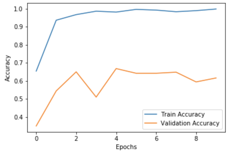
Much better! We’re getting ~65% accuracy on our test set, it’s far from perfect, but it’s much better than using the raw waves. With the help of more data and more fine-tuning to our network we probably can get much better results.

Conclusion

We saw a very basic implementation of voice classification. Representing sound for machine learning is not trivial at all, there are many methods and a lot of research done. Fourier Transform is the very basics of signal processing and is used almost everywhere and is the fundamentals of working with sound.

You can find code with my experiments here.

Next Topics to explore:

• Mel Scale Spectrograms
• Mel-frequency cepstral coefficients (MFCCs)