At its core, Data Science relies on methods of machine learning. But Data Science is also more than just predicting who will buy, who will click or what will break. Data Science uses ML methods and combines them with other methods. In this article, we will discuss Prescriptive Analytics, a technology which combines machine learning with optimization.

Prescriptive Analytics — What to do and not what will happen

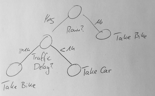
My favorite example of how to explain comes from Ingo Mierswa. Let's say you have a machine learning model which predicts that it will rain tomorrow. Nice — but what does it mean for you? Will you drive to work or will you bike? You could not be the only one who prefers to drive in this case. The result could be, that you are stuckin traffic for an hour. Would it be better to still take the bike, despite the rain?

The solution to this is to define a custom fitness function. You would maximize this fitness for given the weather prediction, the expected traffic and your personal preferences. This is prescriptive analytics! The idea is not to merely forecast what will happen but also advice on what to do.

In this easy example, we have a very small hyperspace of actionable options: Taking the bike or not. This makes our optimization easy: Evaluate both and take the best. In the upcoming real-world example, you can see that this hyperspace can be huge and the optimization problem quite tricky.

Predictive Pricing

You might be tempted to use direct predictive modeling for price calculation. Let's say you have a data set with the correct price. You can treat this as a regression problem and solve using your favorite ML method. The resulting model can then directly be used in production to predict prices.

The big problem here is the miracle to have a label. Where do you get the price from? In practice, you use human-generated prices. How do you know that these are good? You essentially limit the maximum quality of your modeling by the quality of these labels. Of course, you can bootstrap yourself out of this problem by using A/B testing. You would sometimes offer prices which are lower or higher than the human-generated prices and measure success. But this is expensive and not always feasible.

Prescriptive Pricing

Another approach to solve this is Prescriptive Pricing. Similar to the rain-example we need to define a fitness function which reflects the business case. In a retail example, you can start off with the demand-price relationship. An easy fitness function would look like this:

fitness = gain = (Price — Cost)*demand

where demand is the result of a machine learning model which depends on the day, price and maybe even other factors.

If you are working with an insurance provider your fitness will be something like:

fitness = profitability = f(Premium,DefaultRisk,..)

In this example, we want to optimize the premium to have maximum profitability. The other factors are again derived from machine learning models which depend on customer attribute.

Implementation in RapidMiner

Let’s have a look at how to implement such a system. I am employed at RapidMiner and thus my go-to tool is of course RapidMiner. Of course you can build similar things in Python or R if you like.

In our implementation we want to score if customers will accept a given offer. The result is a confidence for acceptance which depends on the price and the other meta data. It’s important to note here, that confidence is not equal to probability, even if it is normalized in [0,1].

In the prescriptive part we will use this model to define our price. We will vary the price in a way, that each customer has a 0.75 confidence of accepting our offer. The 0.75 might be derived from sample constraints. For example, we want to have at least 1000 accepted offers per month. The fitness function we derive from this is:

fitness = price-if([confidence(accept)]<0.75,(0.75-[confidence(accept)])*1e6,0)

meaning we add a penalty factor whenever our confidence drops below our threshold.

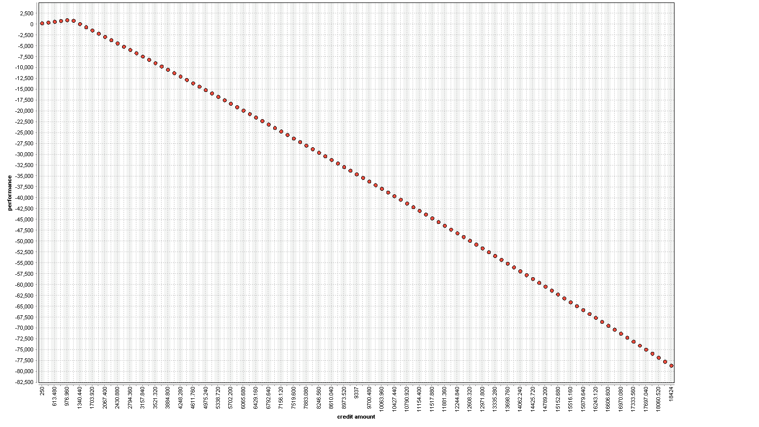
The example process which is depicted above is first deriving a model to predict. Next we run into the optimization. The optimization takes the input example we want to optimize, a reference set to set default bounds and the model. Within the optimization loop we calculate the fitness above. Since the optimization is univariate we can use a grid. We could use CMA-ES, BYOBA or Evolutionary Optimization. The result is a fitness like this

We can see that the fitness rises with increasing price and then drops because the confidence is below 0.75. The derived price is: 976 Euro.

The process depicted here can be found on my github profile.