2. Markov Decision Processes

A Markov Decision Processes (MDP) is a discrete time stochastic control process. MDP is the best approach we have so far to model the complex environment of an AI agent. Every problem that the agent aims to solve can be considered as a sequence of states S1, S2, S3, … Sn

2.1 Markov Processes

A Markov Process is a stochastic model describing a sequence of possible states in which the current state depends on only the previous state. This is also called the Markov Property (Eq. 1). For reinforcement learning it means that the next state of an AI agent only depends on the last state and not all the previous states before.

A Markov Process is a stochastic process. It means that the transition from the current state sto the next state s’ can only happen with a certain probability Pss’ (Eq. 2). In a Markov Process an agent that is told to go left would go left only with a certain probability of e.g. 0.998. With a small probability it is up to the environment to decide where the agent will end up.

Pss’ can be considered as an entry in a state transition matrix P that defines transition probabilities from all states s to all successor states s’ (Eq. 3).

Remember: A Markov Process (or Markov Chain) is a tuple <S, P> . S is a (finite) set of states. P is a state transition probability matrix.

2.2 Markov Reward Process

A Markov Reward Process is a tuple <S, P, R>. Here R is the reward that the agent expects to receive in the state s (Eq. 4). This process is motivated by the fact that for an AI agent that aims to achieve a certain goal e.g. winning a chess game, certain states (game configurations) are more promising than others in terms of strategy and potential to win the game.

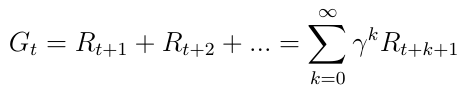
The primary topic of interest is the total reward Gt (Eq. 5) which is the expected accumulated reward the agent will receive across the sequence of all states. Every reward is weighted by so called discount factor γ ∈ [0, 1]. It is mathematically convenient to discount rewards since it avoids infinite returns in cyclic Markov processes. Besides the discount factor means the more we are in the future the less important the rewards become, because the future is often uncertain. If the reward is financial, immediate rewards may earn more interest than delayed rewards. Besides animal/human behavior shows preference for immediate reward.

2.3 Value Function

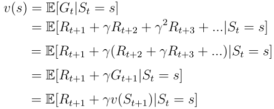
An other important concept is the the one of the value function v(s). The value function maps a value to each state s. The value of a state s is defined as the expected total reward the AI agent will receive if it starts its progress in the state s (Eq. 6).

The value function can be decomposed into two parts:

• The immediate reward R(t+1) the agent receives being in states.
• The discounted value v(s(t+1)) of the next state after the state s.

3. Bellman Equation

3.1 Bellman Equation for Markov Reward Processes

The decomposed value function (Eq. 8) is also called the Bellman Equation for Markov Reward Processes. This function can be visualized in a node graph (Fig. 6). Starting in state s leads to the value v(s). Being in the state s we have certain probability Pss’ to end up in the next state s’. In this particular case we have two possible next states. To obtain the value v(s) we must sum up the values v(s’) of the possible next statesweighted by the probabilities Pss’ and add the immediate reward from being in state s. This yields Eq. 9, which is nothing else than Eq.8 if we execute the expectation operator E in the equation.

3.2 Markov Decision Process — Definition

A Markov Decision Process is a Markov Reward Process with decisions. A Markov Decision Process is described by a set of tuples <S, A, P, R >, A being a finite set of possible actions the agent can take in the state s. Thus the immediate reward from being in state s now also depends on the action a the agent takes in this state (Eq. 10).

3.3 Policies

At this point we shall discuss how the agent decides which action must be taken in a particular state. This is determined by the so called policy π (Eq. 11). Mathematically speaking a policy is a distribution over all actions given a state s. The policy determines the mapping from a state s to the action a that must be taken by the agent.

Remember: Intuitively speaking the policy π can be described as a strategy of the agent to select certain actions depending on the current state s.

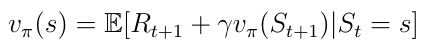
The policy leads to a new definition of the the state-value function v(s) (Eq. 12) which we define now as the expected return starting from state s, and then following a policy π.

3.4 Action-Value Function

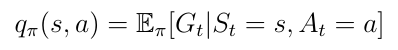
An other important function besides the state-value-function is the so called action-value function q(s,a) (Eq. 13). The action-value function is the expected return we obtain by starting in state s, taking action a and then following a policy π. Notice that for a state s, q(s,a) can take several values since there can be several actions the agent can take in a state s. The calculation of Q(s, a) is achieved by a neural network. Given a state s as input the network calculates the quality for each possible action in this state as a scalar (Fig. 7). Higher quality means a better action with regards to the given objective.

Remember: Action-value function tells us how good is it to take a particular action in a particular state.

Previously the state-value function v(s) could be decomposed into the following form:

The same decomposition can be applied to the action-value function:

At this point lets discuss how v(s) and q(s,a) relate to each other. The relation between these functions can be visualized again in a graph:

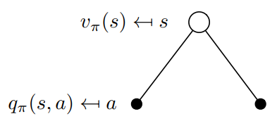
In this example being in the state s allows us to take two possible actions a. By definition taking a particular action in a particular state gives us the action-value q(s,a). The value function v(s) is the sum of possible q(s,a) weighted by the probability (which is non other than the policy π) of taking an action a in the state s (Eq. 16).

Now lets consider the opposite case in Fig. 9. The root of the binary tree is now a state in which we choose to take an particular action a. Remember that the Markov Processes are stochastic. Taking an action does not mean that you will end up where you want to be with 100% certainty. Strictly speaking you must consider probabilities to end up in other states after taking the action. In this particular case after taking action a you can end up in two different next states s’:

To obtain the action-value you must take the discounted state-values weighted by the probabilities Pss’ to end up in all possible states (in this case only 2) and add the immediate reward:

Now that we know the relation between those function we can insert v(s) from Eq. 16 into q(s,a) from Eq. 17. We obtain Eq. 18 and it can be noticed that there is a recursive relation between the current q(s,a) and next action-value q(s’,a’).

This recursive relation can be again visualized in a binary tree (Fig. 10). We begin with q(s,a), end up in the next state s’ with a certain probability Pss’ from there we can take an action a’ with the probability π and we end with the action-value q(s’,a’). To obtain q(s,a) we must go up in the tree and integrate over all probabilities as it can be seen in Eq. 18.

3.5 Optimal Policy

The most important topic of interest in deep reinforcement learning is finding the optimal action-value function q*. Finding q* means that the agent knows exactly the quality of an action in any given state. Furthermore the agent can decide upon the quality which action must be taken. Lets define that q* means. The best possible action-value function is the one that follows the policy that maximizes the action-values:

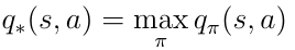
To find the best possible policy we must maximize over q(s, a). Maximization means that we select only the action a from all possible actions for which q(s,a) has the highest value. This yields the following definition for the optimal policy π:

3.6 Bellman Optimality Equation

The condition for the optimal policy can be inserted into Eq. 18. Thus provides us with the Bellman Optimality Equation:

If the AI agent can solve this equation than it basically means that the problem in the given environment is solved. The agent knows in any given state or situation the quality of any possible action with regards to the objective and can behave accordingly.

Solving the Bellman Optimality Equationwill be the topic of the upcoming articles. In the following article I will present you the first technique to solve the equation called Deep Q-Learning.