Feature Selection

While making and adding features is useful to see how different features impact our model, our final result is not necessarily the optimal set of inputs. We may have multicollinearity to address within our features (correlations between features) and others just might not be helpful in our prediction.

There are a few different ways to address feature selection and I tried two different approaches. First was Principal Component Analysis (PCA), which looks to reduce the number of dimensions based on the explained variance of features. This features a two-step process of fitting the PCA with an undefined number of components, analyzing the explained variance, then re-fitting with the smallest number of components that capture the most variance.

pca = PCA()pca.fit(poly_df_s, predict_df.AV_TOTAL)

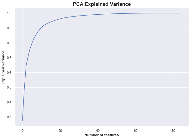
We see that nearly 100% of the variance is explained by about half the features. We can then use dimensionality reduction with PCA and 40 features with the goal of achieving a result similar to that of all features.

fitted_pca = pd.DataFrame(PCA(n_components=40).fit_transform(poly_df_s, predict_df.AV_TOTAL))

Running a model on the PCA-transformed data with 40 components yielded a similar result for the Gradient Boosting algorithm — proving that about half of our features were inconsequential to that model — while the KNeighbors and Random Forest saw slightly decreased performance.

The second approach used the SelectKBest function search for the best features to use. I tested the models against 5 values of k ranging from 20 to the maximum number of columns, and it turned out that 60 produced the best results.

# select_k_best_model_test is a function defined earlier in the code # that fits a SelectKBest model, tests the models on that data, and # returns both the results of the test (MAE, RMSE, score) plus a    # data frame of the condensed columns

k_to_test = [20, 30, 40, 60, 84]for i in k_to_test:        result, df = select_k_best_model_test(i)        print('The results for the best %i features' %i)    print(result)    print('\n')

After fitting the SelectKBest model with 60 columns, I tried to offset the multicollinearity issue by removing correlated columns (which I considered to be those with a correlation above 0.8).

corr_matrix = best_k.corr().abs()## Select upper triangle of correlation matrixupper = corr_matrix.where(np.triu(np.ones(corr_matrix.shape), k=1).astype(np.bool))## Find index of feature columns with correlation greater than 0.8to_drop = [column for column in upper.columns if any(upper[column] > 0.8)]

## Drop columns with a correlation about 0.8  

best_k_consolidated = best_k.drop(to_drop, axis=1)

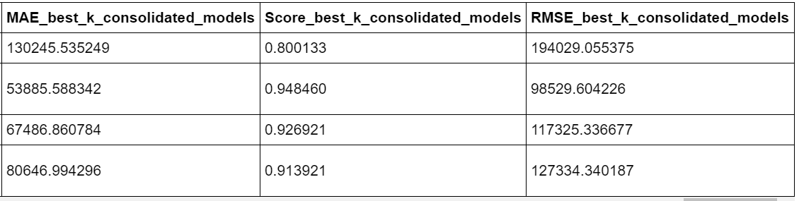
The final result was a model with 37 columns — a sizable reduction from our original 84 — that performed as well or better than any other model. A sampling of the remaining columns includes living area (sq. feet), base floor (i.e. first floor, second, etc.), view (Average, Excellent, etc.), a number of neighborhood dummy variables, and others; about a third of the final columns were a result of our feature engineering and/or bringing in other external data.

Model Tuning

After going through the variable creation and feature selection from those variables, it comes time to see whether we can improve on the out-of-the-box models by tuning the hyperparameters.

I used a combination of GridSearchCV and RandomizedSearchCV depending on the model to search across parameters for the optimal results. These functions either search every combination of parameter inputs (GridSearch) or a set number of randomly selected inputs (RandomizedSearch).

params_grid_gbr = {'loss':['ls','lad','huber'], 'learning_rate':np.arange(0.02, 0.4, 0.03),                    'n_estimators':np.arange(100, 500, 50), 'min_samples_split': np.arange(2, 50, 5),                    'max_depth':np.arange(3, 15, 3)}gbr = GradientBoostingRegressor(random_state=66)    gbr_grid = RandomizedSearchCV(gbr, params_grid_gbr, n_iter=10, cv=5, scoring='neg_mean_absolute_error',)

gbr_grid.fit(tr_x, tr_y)

The result of running these algorithms is, for each model tuned, a set of optimal parameters based on the inputs tested. The caveat here is that the optimal parameters are a function of the parameters that we test, so in effect they could be considered a local optimum instead of a global optimum (i.e. if we were to test every single possible parameter combination).

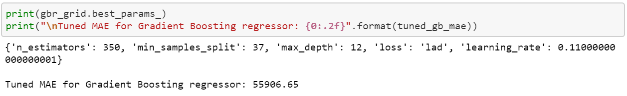
The Gradient Boosting Regressor saw the largest improvement from tuning, with the MAE dropping from ~$80,000 to ~$55,900, an improvement of about 30%! Others, such as the Random Forest, didn’t see any meaningful change with the tuning, while the performance of the KNeighbors as measured by MAE decreased by a little over 6%.

The Outcome

After all of the above, it’s time to look at the outcome of our work. We’ll start by looking at a few metrics, followed by an illustrative visual representation of the errors from one of our models.

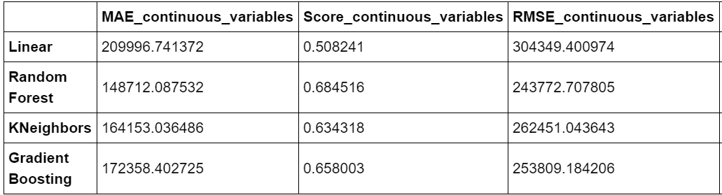
From a naïve “baseline” model that predicts the property value to be the average of all properties, our best prediction decreases the MAE by ~80% from ~$290,000 to ~$53,600. From the first model of continuous variables to the tuned models, the minimum MAE dropped from ~$150,000 to $53,600, a reduction of 64%, and the R2 improved from a range of 0.5-.68 to 0.8–0.95.

The final tuned models had mean absolute error values of:

• Random Forest: $53, 699
• KNeighbors: $63, 230
• Gradient Boosting: $55, 906

Overall, our models deviate from the actual property values by ~10%. Our predictions are by no means perfect, but they’re in the ballpark. I’d be curious to learn the improvements that others could make on top of the process that I’ve undertaken, or what the results would be of more complex models that are beyond my current skills.

The final visual that I’ll provide is examining the errors of one of our models and looking for whether there’s any systematic bias that the model couldn’t capture (e.g. by property value, neighborhood, consistent over/under prediction). The graph below shows the absolute errors for the Random Forest model, colored by neighborhood, with the bubble size being the size of the error (hence the clear area on the 45-degree line through the middle — small error = small bubbles).