How to Build Exponential Smoothing Models Using Python: Simple Exponential Smoothing, Holt, and Holt-Winters

How many iPhone XS will be sold in first 12 months? What’s the demand trend for Tesla after Elon musk smokes weed on a live show? Will this winter be warm? ( I live in Canada.) If you are curious about these problems, Exponential smoothing promises you the possibility of peeking into the future by building models.

Exponential smoothing methods assign exponentially decreasing weights for past observations. The more recent the observation is obtained, the higher weight would be assigned. For example, it is reasonable to attach larger weights to observations from last month than to observations from 12 months ago.

This article will illustrate how to build Simple Exponential Smoothing, Holt, and Holt-Winters models using Python and Statsmodels. For each model, the demonstration is organized in the following way,

Statsmodels is a Python module that provides classes and functions for implementing many different statistical models. We need to import it into Python code as follows.

from statsmodels.tsa.api import ExponentialSmoothing, SimpleExpSmoothing, Holt

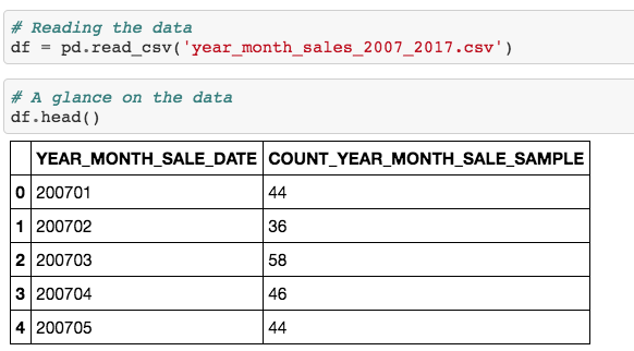
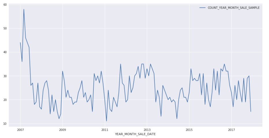
Source dataset in our examples contains the number of property sales in a U.S. town covering the period from 2007-01 to 2017-12.

Use line plot that we can see data variation over years.

df.plot.line(x = 'YEAR_MONTH_SALE_DATE',              y = 'COUNT_YEAR_MONTH_SALE_SAMPLE')plt.show()

We will forecast property sales in 2017 using the 10-year historical data (2007-2016).

Simple Exponential Smoothing (SES)

SES is a good choice for forecasting data with no clear trend or seasonal pattern. Forecasts are calculated using weighted averages, which means the largest weights are associated with most recent observations, while the smallest weights are associated with the oldest observations:

where 0≤ α ≤1 is the smoothing parameter.

The weights decrease rate is controlled by the smoothing parameter α. If α is large (i.e., close to 1), more weight is given to the more recent observations. There are 2 extreme cases:

• α=0: the forecasts of all future values are equal to the average (or “mean”) of the historical data, which is called Average method.
• α=1: simply set all forecasts to be the value of the last observation, which is called Naive method in statistics.

Here we run three variants of simple exponential smoothing:

1. In fit1, we explicitly provide the model with the smoothing parameter α=0.2
2. In fit2, we choose an α=0.6
3. In fit3, we use the auto optimization that allow statsmodels to automatically find an optimized value for us. This is the recommended approach.

# Simple Exponential Smoothingfit1 = SimpleExpSmoothing(saledata).fit(smoothing_level=0.2,optimized=False)fcast1 = fit1.forecast(12).rename(r'$\alpha=0.2$')# plotfcast1.plot(marker='o', color='blue', legend=True)fit1.fittedvalues.plot(marker='o',  color='blue')fit2 = SimpleExpSmoothing(saledata).fit(smoothing_level=0.6,optimized=False)fcast2 = fit2.forecast(12).rename(r'$\alpha=0.6$')# plotfcast2.plot(marker='o', color='red', legend=True)fit2.fittedvalues.plot(marker='o', color='red')fit3 = SimpleExpSmoothing(saledata).fit()fcast3 = fit3.forecast(12).rename(r'$\alpha=%s$'%fit3.model.params['smoothing_level'])# plotfcast3.plot(marker='o', color='green', legend=True)fit3.fittedvalues.plot(marker='o', color='green')plt.show()

Forecasting property sales with SES for the period from 2017-01 to 2017-12.

Holt’s Method

Holt extended simple exponential smoothing (solution to data with no clear trend or seasonality) to allow the forecasting of data with trends in 1957. Holt’s method involves a forecast equation and two smoothing equations (one for the level and one for the trend):

where 0≤ α ≤1 is the level smoothing parameter, and 0≤ β* ≤1 is the trend smoothing parameter.

For long-term forecast, forecasting with Holt’s method will increase or decrease indefinitely into the future. In this case, we use the Damped trend method which has a damping parameter 0< ϕ <1 to prevent the forecast “go wild”.

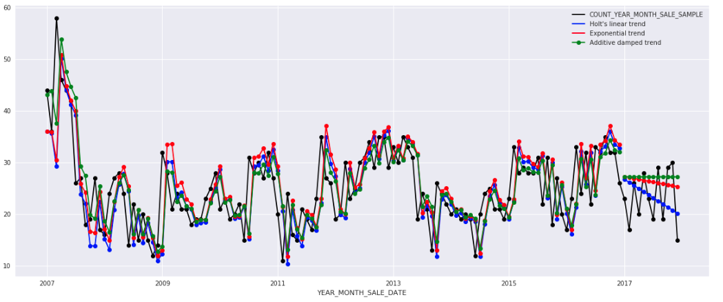
Again, here we run three variants of Halt’s method:

1. In fit1, we explicitly provide the model with the smoothing parameter α=0.8, β*=0.2.
2. In fit2, we use an exponential model rather than a Holt’s additive model(which is default).
3. In fit3, we use a damped version of the Holt’s additive model but allow the dampening parameter ϕ to be optimized while fixing the values for α=0.8, β*=0.2.

fit1 = Holt(saledata).fit(smoothing_level=0.8, smoothing_slope=0.2, optimized=False)fcast1 = fit1.forecast(12).rename("Holt's linear trend")fit2 = Holt(saledata, exponential=True).fit(smoothing_level=0.8, smoothing_slope=0.2, optimized=False)fcast2 = fit2.forecast(12).rename("Exponential trend")fit3 = Holt(saledata, damped=True).fit(smoothing_level=0.8, smoothing_slope=0.2)fcast3 = fit3.forecast(12).rename("Additive damped trend")fit1.fittedvalues.plot(marker="o", color='blue')fcast1.plot(color='blue', marker="o", legend=True)fit2.fittedvalues.plot(marker="o", color='red')fcast2.plot(color='red', marker="o", legend=True)fit3.fittedvalues.plot(marker="o", color='green')fcast3.plot(color='green', marker="o", legend=True)plt.show()

Holt-Winters’ Method

(Peter Winters was a student of Holt. Holt-Winters’ Method was first suggested by Peter, and then they worked on it together. What a beautiful and great connection. Just like Plato met Socrates.)

Holt-Winters’ Method is suitable for data with trends and seasonalities which includes a seasonality smoothing parameter γ. There are two variations to this method:

• Additive method: the seasonal variations are roughly constant through the series.
• Multiplicative method: the seasonal variations are changing proportionally to the level of the series.

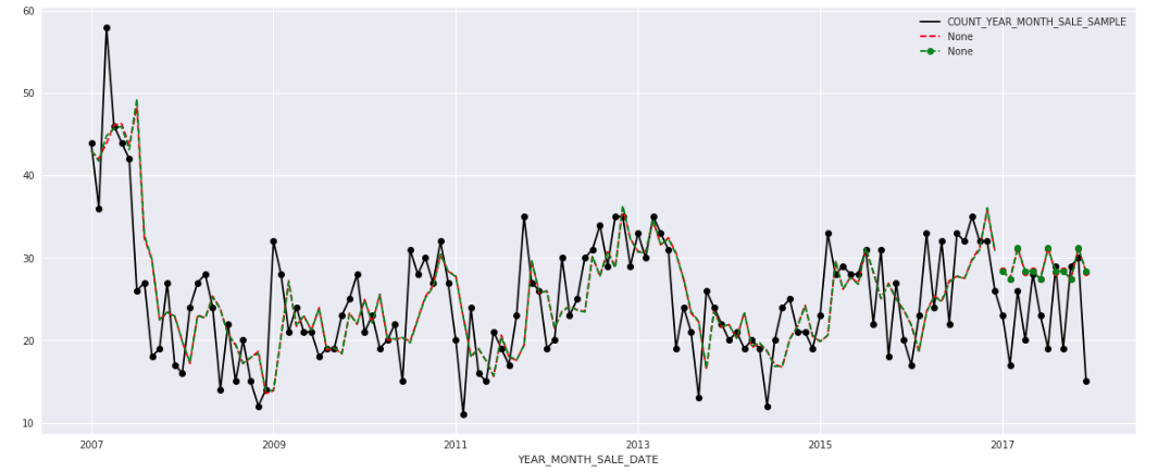
Here, we run full Holt-Winters’ method including a trend component and a seasonal component. Statsmodels allows for all the combinations including as shown in the examples below:

1. In fit1, we use additive trend, additive seasonal of period season_length=4 and a Box-Cox transformation.
2. In fit2, we use additive trend, multiplicative seasonal of period season_length=4 and a Box-Cox transformation.
3. In fit3, we use additive damped trend, additive seasonal of period season_length=4 and a Box-Cox transformation.
4. In fit4, we use additive damped trend, multiplicative seasonal of period season_length=4 and a Box-Cox transformation.

fit1 = ExponentialSmoothing(saledata, seasonal_periods=4, trend='add', seasonal='add').fit(use_boxcox=True)fit2 = ExponentialSmoothing(saledata, seasonal_periods=4, trend='add', seasonal='mul').fit(use_boxcox=True)fit3 = ExponentialSmoothing(saledata, seasonal_periods=4, trend='add', seasonal='add', damped=True).fit(use_boxcox=True)fit4 = ExponentialSmoothing(saledata, seasonal_periods=4, trend='add', seasonal='mul', damped=True).fit(use_boxcox=True)

fit1.fittedvalues.plot(style='--', color='red')fit2.fittedvalues.plot(style='--', color='green')fit1.forecast(12).plot(style='--', marker='o', color='red', legend=True)fit2.forecast(12).plot(style='--', marker='o', color='green', legend=True)plt.show()print("Forecasting sales of properties using Holt-Winters method with both additive and multiplicative seasonality.")

To summarize, we went through mechanics and python code for 3 Exponential smoothing models. As the table below shows, I provide a methodology for selecting an appropriate model for your dataset.

A summary of smoothing parameters for different component forms of Exponential smoothing methods.

Exponential smoothing is one of the most widely used and successful forecasting methods in the industry nowadays. How to forecast retail sales, tourists’ arrivals, electricity demand, or revenue growth? Exponential smoothing is one of the superpowers you need to reveal the future in front of you.