Three Popular Clustering Methods and When to Use Each

In the mad rush to find new ways of teasing apart labeled data, we often forget about everything we can do with unsupervised learning. Unsupervised machine learning can be very powerful in its own right, and clustering is by far the most common expression of this group of problems.

This is a quick run-down of three of the most popular clustering approaches and what types of situations each is best-suited to. The one thing clustering has in common with supervised problems is that there is no silver bullet; each algorithm will have its time and place depending on what you’re trying to accomplish. This should give you some intuition as far as when to use each, with only a smidge of math.

Hierarchical Clustering

Imagine you have some number of clusters k you’re interested in finding. All you know is that you can probably break up your dataset into that many distinct groups at the top level, but you might also be interested in the groups inside your groups, or the groups inside of those groups. To get that kind of structure, we use hierarchical clustering.

We begin with n different points and k different clusters we want to discover; for our purposes, n = 4, and k = 2.

Start by treating each point as if it were its own cluster.

We then start merging each of our single-point clusters into larger clusters, using the clusters that are closest together. We find the smallest distance from the pairwise distance matrix — which is just a table of the distance of every cluster from every other cluster.

This is initialized as the Euclidean distance between each point, but after that, we switch to one of a variety of different ways of measuring cluster distance. If you’re interested in learning more about these techniques, look up single link clustering, complete link clustering, clique margins, and Ward’s Method.

Anyways, we start merging the clusters that are closest together. Say we know that x1 and x3are closest together. We then merge those two into a new cluster, ca.

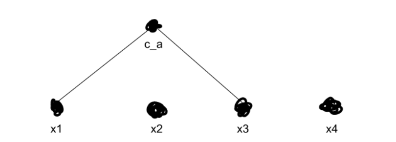
We now recalculate ca’s distance from every other cluster, using whichever method we prefer from the aforementioned grab-bag. Then we repeat, merging our clusters over and over until we get k top-level clusters — in our example, two clusters. Say we figure out that x2 is closer to ca than to x4.

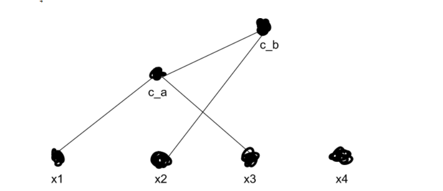
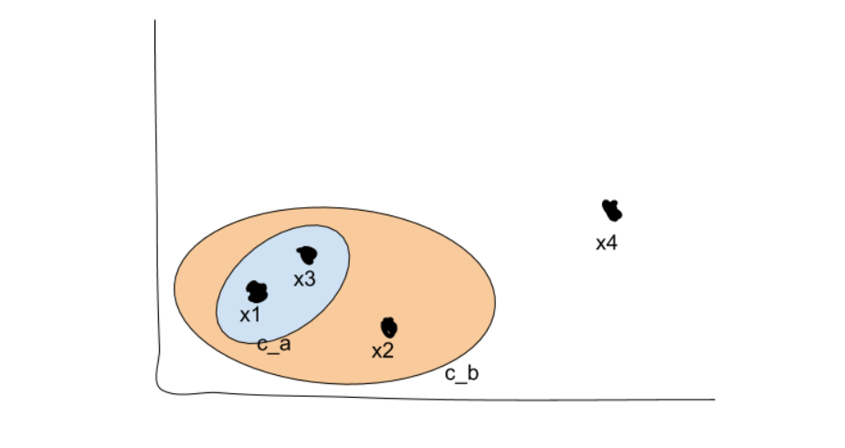
We now have two top-level clusters, cb and x4 (remember that each point starts as its own cluster). We can now search the tree structure we’ve created to search for sub-clusters, which in our original 2-D view would look like this:

Density-Based Clustering

Hierarchical clustering is advantageous for understanding any hidden structures in your data, but it has a major pitfall. In the version shown above, we assume that every data point is relevant — which is almost never the case in the real world.

Density-based clustering methods provide a safety valve. Instead of assuming that every point is part of some cluster, we only look at points that are tightly packed and assume everything else is noise.

This approach requires two parameters: a radius ? and a neighborhood density ?. For every point, we calculate Neps(x) — the number of points that are at most ? away from x. If Neps(x) ≥ ?, not counting x, then x is considered a core point. If a point isn’t a core point, but it is a member of a core point’s neighborhood, then it is considered a border point. Everything else is just considered noise.

One of the most common and, indeed, performative implementations of density-based clustering is Density-based Spatial Clustering of Applications with Noise, better known as DBSCAN. DBSCAN works by running a connected components algorithm across the different core points. If two core points share border points, or a core point is a border point in another core point’s neighborhood, then they’re part of the same connected component, which forms a cluster.

Say we have a relatively small ? and a decently large ?. We might wind up with clusters like this:

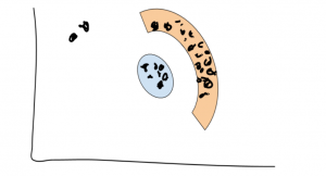
See? Those two lonely points are very far away from the two clusters, and there are too few for them to really mean anything — so they’re just noise.

Notice that we’re also able to discover non-convex clusters this way (see the orange arc). Pretty neat!

We don’t need to specify a number of clusters we’re interested in for density-based clustering to work — it will automatically discover some number of clusters based on your ? and ?. This is especially useful when you expect all of your clusters to have a similar density.

K-Means Clustering

Hierarchical clustering excels at discovering embedded structures in the data, and density-based approaches excel at finding an unknown number of clusters of similar density. However, both fail at finding a ‘consensus’ across the full dataset. Hierarchical clustering can put together clusters that seem close, but no information about other points is considered. Density-based methods only look at a small neighborhood of nearby points and similarly fail to consider the full dataset.

That’s where K-means clustering comes in. In a sense, K-means considers every point in the dataset and uses that information to evolve the clustering over a series of iterations.

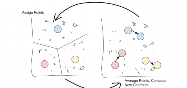
K-means works by selecting k central points, or means, hence K-Means. These means are then used as the centroid of their cluster: any point that is closest to a given mean is assigned to that mean’s cluster.

Once all points are assigned, move through each cluster and take the average of all points it contains. This new ‘average’ point is the new mean of the cluster.

Just repeat these two steps over and over again until the point assignments stop changing!

Once the point assignments have stopped changing, the algorithm is said to have converged.

We will now have k different clusters, each of which has a centroid closer to every point in its cluster than any other centroid. Calculating the centroid again won’t change the assignments, so we stop. That’s really all there is to K-means, but it’s a very powerful method for finding a known number of clusters while considering the entire dataset.

There are numerous approaches to initializing your means. The Forgy Method randomly selects k random observations from the data and uses these as the starting points. The Random Partition Method will assign every point in the dataset to a random cluster, then calculate the centroid from these and resume the algorithm.

While K-means is an NP-hard problem, heuristic methods are capable of finding decent approximations to the global optimum in polynomial time and are able to handle big datasets efficiently, making it a solid choice over hierarchical clustering in some cases.

Clustering is a strange world, with an even stranger collection of techniques. These three approaches are only some of the most popular, but they will get you a long way in discovering unknown groupings in your data. Clustering is very useful in exploratory data analysis, finding initialization points for other analyses, and is also incredibly simple to deploy. Used wisely, clustering can provide surprising insights into your data. Consider it another notch in your belt.