It is sometimes said that Python, compared to low-level languages such as C++, improves development time at the expense of runtime. Fortunately, there are a handful of ways to speed up operation runtime in Python without sacrificing ease of use. One option suited for fast numerical operations is NumPy, which deservedly bills itself as the fundamental package for scientific computing with Python.

Granted, few people would categorize something that takes 50 microseconds (fifty millionths of a second) as “slow.” However, computers might beg to differ. The runtime of an operation taking 50 microseconds (50 μs) falls under the realm of microperformance, which can loosely be defined as operations with a runtime between 1 microsecond and 1 millisecond.

Why does speed matter? The reason that microperformance is worth monitoring is that small differences in runtime become amplified with repeated function calls: an incremental 50 μs of overhead, repeated over 1 million function calls, translates to 50 seconds of incremental runtime.

When it comes to computation, there are really three concepts that lend NumPy its power:

• Vectorization
• Broadcasting
• Indexing

In this tutorial, you’ll see step by step how to take advantage of vectorization and broadcasting, so that you can use NumPy to its full capacity. While you will use some indexing in practice here, NumPy’s complete indexing schematics, which extend Python’s slicing syntax, are their own beast. If you’re looking to read more on NumPy indexing, grab some coffee and head to the Indexing section in the NumPy docs.

Free Bonus: Click here to get access to a free NumPy Resources Guide that points you to the best tutorials, videos, and books for improving your NumPy skills.

Getting into Shape: Intro to NumPy Arrays

The fundamental object of NumPy is its ndarray (or numpy.array), an n-dimensional array that is also present in some form in array-oriented languages such as Fortran 90, R, and MATLAB, as well as predecessors APL and J.

Let’s start things off by forming a 3-dimensional array with 36 elements:

>>> import numpy as np

>>> arr = np.arange(36).reshape(3, 4, 3)
>>> arr
array([[[ 0,  1,  2],
        [ 3,  4,  5],
        [ 6,  7,  8],
        [ 9, 10, 11]],

       [[12, 13, 14],
        [15, 16, 17],
        [18, 19, 20],
        [21, 22, 23]],

       [[24, 25, 26],
        [27, 28, 29],
        [30, 31, 32],
        [33, 34, 35]]])

Picturing high-dimensional arrays in two dimensions can be difficult. One intuitive way to think about an array’s shape is to simply “read it from left to right.” arr is a 3 by 4 by 3 array:

>>> arr.shape
(3, 4, 3)

Visually, arr could be thought of as a container of three 4x3 grids (or a rectangular prism) and would look like this:

Higher dimensional arrays can be tougher to picture, but they will still follow this “arrays within an array” pattern.

Where might you see data with greater than two dimensions?

• Panel data can be represented in three dimensions. Data that tracks attributes of a cohort (group) of individuals over time could be structured as (respondents, dates, attributes). The 1979 National Longitudinal Survey of Youth follows 12,686 respondents over 27 years. Assuming that you have ~500 directly asked or derived data points per individual, per year, this data would have shape (12686, 27, 500) for a total of 177,604,000 data points.
• Color-image data for multiple images is typically stored in four dimensions. Each image is a three-dimensional array of (height, width, channels), where the channels are usually red, green, and blue (RGB) values. A collection of images is then just (image_number, height, width, channels). One thousand 256x256 RGB images would have shape (1000, 256, 256, 3). (An extended representation is RGBA, where the A–alpha–denotes the level of opacity.)

For more detail on real-world examples of high-dimensional data, see Chapter 2 of François Chollet’s Deep Learning with Python.

What is Vectorization?

Vectorization is a powerful ability within NumPy to express operations as occurring on entire arrays rather than their individual elements. Here’s a concise definition from Wes McKinney:

This practice of replacing explicit loops with array expressions is commonly referred to as vectorization. In general, vectorized array operations will often be one or two (or more) orders of magnitude faster than their pure Python equivalents, with the biggest impact [seen] in any kind of numerical computations. [source]

When looping over an array or any data structure in Python, there’s a lot of overhead involved. Vectorized operations in NumPy delegate the looping internally to highly optimized C and Fortran functions, making for cleaner and faster Python code.

Counting: Easy as 1, 2, 3…

As an illustration, consider a 1-dimensional vector of True and False for which you want to count the number of “False to True” transitions in the sequence:

>>> np.random.seed(444)

>>> x = np.random.choice([False, True], size=100000)
>>> x
array([ True, False,  True, ...,  True, False,  True])

With a Python for-loop, one way to do this would be to evaluate, in pairs, the truth value of each element in the sequence along with the element that comes right after it:

>>> def count_transitions(x) -> int:
...     count = 0
...     for i, j in zip(x[:-1], x[1:]):
...         if j and not i:
...             count += 1
...     return count
...
>>> count_transitions(x)
24984

In vectorized form, there’s no explicit for-loop or direct reference to the individual elements:

>>> np.count_nonzero(x[:-1] < x[1:])
24984

How do these two equivalent functions compare in terms of performance? In this particular case, the vectorized NumPy call wins out by a factor of about 70 times:

>>> from timeit import timeit
>>> setup = 'from __main__ import count_transitions, x; import numpy as np'
>>> num = 1000
>>> t1 = timeit('count_transitions(x)', setup=setup, number=num)
>>> t2 = timeit('np.count_nonzero(x[:-1] < x[1:])', setup=setup, number=num)
>>> print('Speed difference: {:0.1f}x'.format(t1 / t2))
Speed difference: 71.0x

Technical Detail: Another term is vector processor, which is related to a computer’s hardware. When I speak about vectorization here, I’m referring to concept of replacing explicit for-loops with array expressions, which in this case can then be computed internally with a low-level language.

Buy Low, Sell High

Here’s another example to whet your appetite. Consider the following classic technical interview problem:

Given a stock’s price history as a sequence, and assuming that you are only allowed to make one purchase and one sale, what is the maximum profit that can be obtained? For example, given prices = (20, 18, 14, 17, 20, 21, 15), the max profit would be 7, from buying at 14 and selling at 21.

(To all of you finance people: no, short-selling is not allowed.)

There is a solution with n-squared time complexity that consists of taking every combination of two prices where the second price “comes after” the first and determining the maximum difference.

However, there is also an O(n) solution that consists of iterating through the sequence just once and finding the difference between each price and a running minimum. It goes something like this:

>>> def profit(prices):
...     max_px = 0
...     min_px = prices[0]
...     for px in prices[1:]:
...         min_px = min(min_px, px)
...         max_px = max(px - min_px, max_px)
...     return max_px

>>> prices = (20, 18, 14, 17, 20, 21, 15)
>>> profit(prices)
7

Can this be done in NumPy? You bet. But first, let’s build a quasi-realistic example:

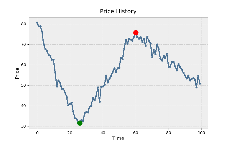
# Create mostly NaN array with a few 'turning points' (local min/max).
>>> prices = np.full(100, fill_value=np.nan)
>>> prices[[0, 25, 60, -1]] = [80., 30., 75., 50.]

# Linearly interpolate the missing values and add some noise.
>>> x = np.arange(len(prices))
>>> is_valid = ~np.isnan(prices)
>>> prices = np.interp(x=x, xp=x[is_valid], fp=prices[is_valid])
>>> prices += np.random.randn(len(prices)) * 2

Here’s what this looks like with matplotlib. The adage is to buy low (green) and sell high (red):

>>> import matplotlib.pyplot as plt

# Warning! This isn't a fully correct solution, but it works for now.
# If the absolute min came after the absolute max, you'd have trouble.
>>> mn = np.argmin(prices)
>>> mx = mn + np.argmax(prices[mn:])
>>> kwargs = {'markersize': 12, 'linestyle': ''}

>>> fig, ax = plt.subplots()
>>> ax.plot(prices)
>>> ax.set_title('Price History')
>>> ax.set_xlabel('Time')
>>> ax.set_ylabel('Price')
>>> ax.plot(mn, prices[mn], color='green', **kwargs)
>>> ax.plot(mx, prices[mx], color='red', **kwargs)

What does the NumPy implementation look like? While there is no np.cummin() “directly,” NumPy’s universal functions (ufuncs) all have an accumulate() method that does what its name implies:

>>> cummin = np.minimum.accumulate

Extending the logic from the pure-Python example, you can find the difference between each price and a running minimum (element-wise), and then take the max of this sequence:

>>> def profit_with_numpy(prices):
...     """Price minus cumulative minimum price, element-wise."""
...     prices = np.asarray(prices)
...     return np.max(prices - cummin(prices))

>>> profit_with_numpy(prices)
44.2487532293278
>>> np.allclose(profit_with_numpy(prices), profit(prices))
True

How do these two operations, which have the same theoretical time complexity, compare in actual runtime? First, let’s take a longer sequence. (This doesn’t necessarily need to be a time series of stock prices at this point.)

>>> seq = np.random.randint(0, 100, size=100000)
>>> seq
array([ 3, 23,  8, 67, 52, 12, 54, 72, 41, 10, ..., 46,  8, 90, 95, 93,
       28, 24, 88, 24, 49])

Now, for a somewhat unfair comparison:

>>> setup = ('from __main__ import profit_with_numpy, profit, seq;'
...          ' import numpy as np')
>>> num = 250
>>> pytime = timeit('profit(seq)', setup=setup, number=num)
>>> nptime = timeit('profit_with_numpy(seq)', setup=setup, number=num)
>>> print('Speed difference: {:0.1f}x'.format(pytime / nptime))
Speed difference: 76.0x

Above, treating profit_with_numpy() as pseudocode (without considering NumPy’s underlying mechanics), there are actually three passes through a sequence:

• cummin(prices) has O(n) time complexity
• prices - cummin(prices) is O(n)
• max(...) is O(n)

This reduces to O(n), because O(3n) reduces to just O(n)–the n “dominates” as n approaches infinity.

Therefore, these two functions have equivalent worst-case time complexity. (Although, as a side note, the NumPy function comes with significantly more space complexity.) But that is probably the least important takeaway here. One lesson is that, while theoretical time complexity is an important consideration, runtime mechanics can also play a big role. Not only can NumPy delegate to C, but with some element-wise operations and linear algebra, it can also take advantage of computing within multiple threads. But there are a lot of factors at play here, including the underlying library used (BLAS/LAPACK/Atlas), and those details are for a whole ‘nother article entirely.

Intermezzo: Understanding Axes Notation

In NumPy, an axis refers to a single dimension of a multidimensional array:

>>> arr = np.array([[1, 2, 3],
...                 [10, 20, 30]])
>>> arr.sum(axis=0)
array([11, 22, 33])
>>> arr.sum(axis=1)
array([ 6, 60])

The terminology around axes and the way in which they are described can be a bit unintuitive. In the documentation for Pandas (a library built on top of NumPy), you may frequently see something like:

axis : {'index' (0), 'columns' (1)}

You could argue that, based on this description, the results above should be “reversed.” However, the key is that axis refers to the axis along which a function gets called. This is well articulated by Jake VanderPlas:

The way the axis is specified here can be confusing to users coming from other languages. The axis keyword specifies the dimension of the array that will be collapsed, rather than the dimension that will be returned. So, specifying axis=0 means that the first axis will be collapsed: for two-dimensional arrays, this means that values within each column will be aggregated. [source]

In other words, summing an array for axis=0 collapses the rows of the array with a column-wise computation.

With this distinction in mind, let’s move on to explore the concept of broadcasting.

Broadcasting

Broadcasting is another important NumPy abstraction. You’ve already seen that operations between two NumPy arrays (of equal size) operate element-wise:

>>> a = np.array([1.5, 2.5, 3.5])
>>> b = np.array([10., 5., 1.])
>>> a / b
array([0.15, 0.5 , 3.5 ])

But, what about unequally sized arrays? This is where broadcasting comes in:

The term broadcasting describes how NumPy treats arrays with different shapes during arithmetic operations. Subject to certain constraints, the smaller array is “broadcast” across the larger array so that they have compatible shapes. Broadcasting provides a means of vectorizing array operations so that looping occurs in C instead of Python. [source]

The way in which broadcasting is implemented can become tedious when working with more than two arrays. However, if there are just two arrays, then their ability to be broadcasted can be described with two short rules:

When operating on two arrays, NumPy compares their shapes element-wise. It starts with the trailing dimensions and works its way forward. Two dimensions are compatible when:

1. they are equal, or
2. one of them is 1

That’s all there is to it.

Let’s take a case where we want to subtract each column-wise mean of an array, element-wise:

>>> sample = np.random.normal(loc=[2., 20.], scale=[1., 3.5],
...                           size=(3, 2))
>>> sample
array([[ 1.816 , 23.703 ],
       [ 2.8395, 12.2607],
       [ 3.5901, 24.2115]])

In statistical jargon, sample consists of two samples (the columns) drawn independently from two populations with means of 2 and 20, respectively. The column-wise means should approximate the population means (albeit roughly, because the sample is small):

>>> mu = sample.mean(axis=0)
>>> mu
array([ 2.7486, 20.0584])

Now, subtracting the column-wise means is straightforward because broadcasting rules check out:

>>> print('sample:', sample.shape, '| means:', mu.shape)
sample: (3, 2) | means: (2,)

>>> sample - mu
array([[-0.9325,  3.6446],
       [ 0.091 , -7.7977],
       [ 0.8416,  4.1531]])

Here’s an illustration of subtracting out column-wise means, where a smaller array is “stretched” so that it is subtracted from each row of the larger array:

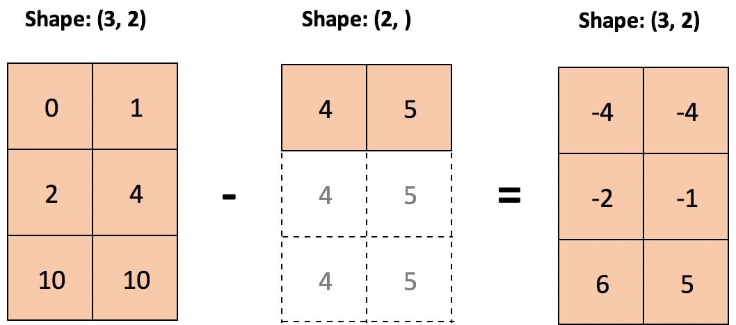
Technical Detail: The smaller-sized array or scalar is not literally stretched in memory: it is the computation itself that is repeated.

This extends to standardizing each column as well, making each cell a z-score relative to its respective column:

>>> (sample - sample.mean(axis=0)) / sample.std(axis=0)
array([[-1.2825,  0.6605],
       [ 0.1251, -1.4132],
       [ 1.1574,  0.7527]])

However, what if you want to subtract out, for some reason, the row-wise minimums? You’ll run into a bit of trouble:

>>> sample - sample.min(axis=1)
ValueError: operands could not be broadcast together with shapes (3,2) (3,)

The problem here is that the smaller array, in its current form, cannot be “stretched” to be shape-compatible with sample. You actually need to expand its dimensionality to meet the broadcasting rules above:

>>> sample.min(axis=1)[:, None]  # 3 minimums across 3 rows
array([[1.816 ],
       [2.8395],
       [3.5901]])

>>> sample - sample.min(axis=1)[:, None]
array([[ 0.    , 21.887 ],
       [ 0.    ,  9.4212],
       [ 0.    , 20.6214]])

Note: [:, None] is a means by which to expand the dimensionality of an array, to create an axis of length one. np.newaxis is an alias for None.

There are some significantly more complex cases, too. Here’s a more rigorous definition of when any arbitrary number of arrays of any shape can be broadcast together:

A set of arrays is called “broadcastable” to the same shape if the following rules produce a valid result, meaning one of the following is true:

1. The arrays all have exactly the same shape.

2. The arrays all have the same number of dimensions, and the length of each dimension is either a common length or 1.

3. The arrays that have too few dimensions can have their shapes prepended with a dimension of length 1 to satisfy property #2.

This is easier to walk through step by step. Let’s say you have the following four arrays:

>>> a = np.sin(np.arange(10)[:, None])
>>> b = np.random.randn(1, 10)
>>> c = np.full_like(a, 10)
>>> d = 8

Before checking shapes, NumPy first converts scalars to arrays with one element:

>>> arrays = [np.atleast_1d(arr) for arr in (a, b, c, d)]
>>> for arr in arrays:
...     print(arr.shape)
...
(10, 1)
(1, 10)
(10, 1)
(1,)

Now we can check criterion #1. If all of the arrays have the same shape, a set of their shapes will condense down to one element, because the set() constructor effectively drops duplicate items from its input. This criterion is clearly not met:

>>> len(set(arr.shape for arr in arrays)) == 1
False

The first part of criterion #2 also fails, meaning the entire criterion fails:

>>> len(set((arr.ndim) for arr in arrays)) == 1
False

The final criterion is a bit more involved:

The arrays that have too few dimensions can have their shapes prepended with a dimension of length 1 to satisfy property #2.

To codify this, you can first determine the dimensionality of the highest-dimension array and then prepend ones to each shape tuple until all are of equal dimension:

>>> maxdim = max(arr.ndim for arr in arrays)  # Maximum dimensionality
>>> shapes = np.array([(1,) * (maxdim - arr.ndim) + arr.shape
...                    for arr in arrays])
>>> shapes
array([[10,  1],
       [ 1, 10],
       [10,  1],
       [ 1,  1]])

Finally, you need to test that the length of each dimension is either (drawn from) a common length, or 1. A trick for doing this is to first mask the array of “shape-tuples” in places where it equals one. Then, you can check if the peak-to-peak (np.ptp()) column-wise differences are all zero:

>>> masked = np.ma.masked_where(shapes == 1, shapes)
>>> np.all(masked.ptp(axis=0) == 0)  # ptp: max - min
True

Encapsulated in a single function, this logic looks like this:

>>> def can_broadcast(*arrays) -> bool:
...     arrays = [np.atleast_1d(arr) for arr in arrays]
...     if len(set(arr.shape for arr in arrays)) == 1:
...         return True
...     if len(set((arr.ndim) for arr in arrays)) == 1:
...         return True
...     maxdim = max(arr.ndim for arr in arrays)
...     shapes = np.array([(1,) * (maxdim - arr.ndim) + arr.shape
...                        for arr in arrays])
...     masked = np.ma.masked_where(shapes == 1, shapes)
...     return np.all(masked.ptp(axis=0) == 0)
...
>>> can_broadcast(a, b, c, d)
True

Luckily, you can take a shortcut and use np.broadcast() for this sanity-check, although it’s not explicitly designed for this purpose:

>>> def can_broadcast(*arrays) -> bool:
...     try:
...         np.broadcast(*arrays)
...         return True
...     except ValueError:
...         return False
...
>>> can_broadcast(a, b, c, d)
True

For those interested in digging a little deeper, PyArray_Broadcast is the underlying C function that encapsulates broadcasting rules.

Array Programming in Action: Examples

In the following 3 examples, you’ll put vectorization and broadcasting to work with some real-world applications.

Clustering Algorithms

Machine learning is one domain that can frequently take advantage of vectorization and broadcasting. Let’s say that you have the vertices of a triangle (each row is an x, y coordinate):

>>> tri = np.array([[1, 1],
...                 [3, 1],
...                 [2, 3]])

The centroid of this “cluster” is an (x, y) coordinate that is the arithmetic mean of each column:

>>> centroid = tri.mean(axis=0)
>>> centroid
array([2.    , 1.6667])

It’s helpful to visualize this:

>>> trishape = plt.Polygon(tri, edgecolor='r', alpha=0.2, lw=5)
>>> _, ax = plt.subplots(figsize=(4, 4))
>>> ax.add_patch(trishape)
>>> ax.set_ylim([.5, 3.5])
>>> ax.set_xlim([.5, 3.5])
>>> ax.scatter(*centroid, color='g', marker='D', s=70)
>>> ax.scatter(*tri.T, color='b',  s=70)

Many clustering algorithms make use of Euclidean distances of a collection of points, either to the origin or relative to their centroids.

In Cartesian coordinates, the Euclidean distance between points p and q is:

So for the set of coordinates in tri from above, the Euclidean distance of each point from the origin (0, 0) would be:

>>> np.sum(tri**2, axis=1) ** 0.5  # Or: np.sqrt(np.sum(np.square(tri), 1))
array([1.4142, 3.1623, 3.6056])

You may recognize that we are really just finding Euclidean norms:

>&g