In most Supervised Machine Learning problems we need to define a model and estimate its parameters based on a training dataset. A popular and easy-to-use technique to calculate those parameters is to minimize model’s error with Gradient Descent. The Gradient Descent estimates the weights of the model in many iterations by minimizing a cost function at every step.

The Gradient Descent Algorithm

Here is the algorithm:

Repeat until convergence {

     Wj = Wj - λ θF(Wj)/θWj

}

Where Wj is one of our parameters (or a vector with our parameters), F is our cost function (estimates the errors of our model), θF(Wj)/θWj is its first derivative with respect to Wj and λ is the learning rate.

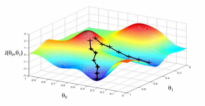
If our F is monotonic, this method will give us after many iterations an estimation of the Wj weights which minimize the cost function. Note that if the derivative is not monotonic we might be trapped to local minimum. In that case an easy way to detect this is by repeating the process for different initial Wj values and comparing the value of the cost function for the new estimated parameters.

Gradient Descent is not always the best method to calculate the weights, nevertheless it is a relatively fast and easy method. If you want to read more about Gradient Descent check out the notes of Ng for Stanford’s Machine Learning course.

Tuning the learning rate

In order for Gradient Descent to work we must set the λ (learning rate) to an appropriate value. This parameter determines how fast or slow we will move towards the optimal weights. If the λ is very large we will skip the optimal solution. If it is too small we will need too many iterations to converge to the best values. So using a good λ is crucial.

Adapting the value of learning rate for different dataset sizes

Depending on the cost function F that we will select, we might face different problems. When the Sum of Squared Errors is selected as our cost function then the value of θF(Wj)/θWj gets larger and larger as we increase the size of the training dataset. Thus the λ must be adapted to significantly smaller values.

One way to resolve this problem is to divide the λ with 1/N, where N is the size of the training data. So the update step of the algorithm can be rewritten as:

Wj = Wj - (λ/N)*θF(Wj)/θWj

Finally another way to resolve this problem is by selecting a cost function that is not affected by the number of train examples that we use, such as the Mean Squared Errors.

Adapting learning rate in each iteration

Another good technique is to adapt the value of λ in each iteration. The idea behind this is that the farther you are from optimal values the faster you should move towards the solution and thus the value of λ should be larger. The closer you get to the solution the smaller its value should be. Unfortunately since you don’t know the actual optimal values, you also don’t know how close you are to them in each step.

To resolve this you can check the value of the error function by using the estimated parameters of the model at the end of each iteration. If your error rate was reduced since the last iteration, you can try increasing the learning rate by 5%. If your error rate was actually increased (meaning that you skipped the optimal point) you should reset the values of Wj to the values of the previous iteration and decrease the learning rate by 50%. This technique is called Bold Driver.

Extra tip: Normalize your Input Vectors

In many machine learning problems normalizing the input vectors is a pretty common practice. In some techniques normalization is required because they internally use distances or feature variances and thus without normalization the results would be heavily affected by the feature with the largest variance or scale. Normalizing your inputs can also help your numerical optimization method (such as Gradient Descent) converge much faster and accurately.

Even though there are several ways to normalize a variable, the [0,1] normalization (also known as min-max) and the z-score normalization are two of the most widely used. Here is how you can calculate both of them:

XminmaxNorm = (X - min(X))/(max(X)-min(X));
XzscoreNorm = (X - mean(X))/std(X);

Hope this works for you!