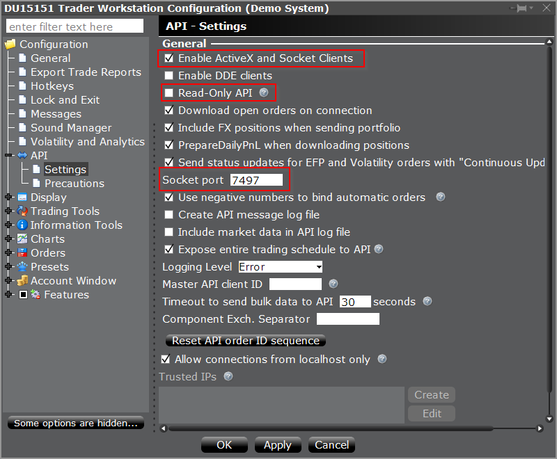
With the client running, we additionally need to do a couple of things

• Under File -> Global Configuration choose Settings -> API and
• Check Enable ActiveX and Socket Clients and uncheck Read-Only API
• Notice that the port is 7497 , which differs from the standard 7496 which is used for Live Trading (remember we chose Paper Trading above)

We are good to go.

Getting a data stream

Let’s start easy by getting a data stream with a simple script

from __future__ import (absolute_import, division, print_function,
                        unicode_literals)

import backtrader as bt

class St(bt.Strategy):
    def logdata(self):
        txt = []
        txt.append('{}'.format(len(self)))
           
        txt.append('{}'.format(
            self.data.datetime.datetime(0).isoformat())
        )
        txt.append('{:.2f}'.format(self.data.open[0]))
        txt.append('{:.2f}'.format(self.data.high[0]))
        txt.append('{:.2f}'.format(self.data.low[0]))
        txt.append('{:.2f}'.format(self.data.close[0]))
        txt.append('{:.2f}'.format(self.data.volume[0]))
        print(','.join(txt))

    def next(self):
        self.logdata()

def run(args=None):
    cerebro = bt.Cerebro(stdstats=False)
    store = bt.stores.IBStore(port=7497)

    data = store.getdata(dataname='TWTR',
                         timeframe=bt.TimeFrame.Ticks)    
    cerebro.resampledata(data, timeframe=bt.TimeFrame.Seconds,
                         compression=10)
    cerebro.addstrategy(St)

    cerebro.run()

if __name__ == '__main__':
    run()

Some notes

• We have chosen TWTR as the ticker (dataname='TWTR' )
• We have applied a timeframe=bt.TimeFrame.Ticks because we want to collect real-time data in the form of ticks. Interactive Brokers doesn’t deliver ready-made 10-seconds bars when they are complete
• The ticks are resample to 10-seconds bars with cerebro.resampledata
• Our strategy class, does simply print the data. Let’s see how it looks like

pipenv run ./ibtutorial.py

Server Version: 76
TWS Time at connection:20180301 10:46:18 CET
1,2018-03-01T06:46:20,33.41,33.43,33.38,33.38,11.00
2,2018-03-01T06:46:30,33.42,33.42,33.34,33.42,15.00
...
1079,2018-03-01T09:46:00,33.56,33.57,33.54,33.57,33.00
1080,2018-03-01T09:46:10,33.56,33.59,33.55,33.57,32.00
1081,2018-03-01T09:46:30,33.44,33.44,33.43,33.43,7.00
1082,2018-03-01T09:46:40,33.44,33.47,33.41,33.44,22.00

Very quickly a whooping total of 1082 bars. This is so, because backtrader has done back-filling for us. But we don’t know where is the difference between back-filled bars and the real-time bars. Let’s rely on notifications by extending our strategy class with this method (and an attribute to control when data is live)

data_live = False

def notify_data(self, data, status, *args, **kwargs):
    print('*' * 5, 'DATA NOTIF:', data._getstatusname(status),
          *args)
    if status == data.LIVE:
        self.data_live = True

And we give ourselves a chance to see the notification

pipenv run ./ibtutorial.py

Server Version: 76
TWS Time at connection:20180301 10:52:58 CET
***** DATA NOTIF: DELAYED
1,2018-03-01T06:53:00,33.43,33.44,33.43,33.43,10.00
...
1081,2018-03-01T09:53:00,33.51,33.51,33.51,33.51,6.00
***** DATA NOTIF: LIVE
1082,2018-03-01T09:53:10,33.52,33.54,33.52,33.52,31.00

Now we see it clearly. At the beginning the data is DELAYED and only after 1081 bars is the system in a position to provide you with real-time data. Remember we are using 10-seconds bars. When we get bar 1082, this is the summary of the last 10 seconds.

Doing some trading

The next step is obviously doing some trading, now that we are getting some data. If you have carefully read the code above you will have noticed that the data stream is fetched with a: store.getdata(...) . And that before that we created the store with store = bt.stores.IBStore(...)

backtrader offers the Store concept to provide a unified interface to access data instances and broker instances. This post is about Interactive Brokers. If you decide to go some other path, you simply need to change the Store. Getting the data will still be done with data = store.getdata(...)

All this store applies to the broker and will be used now. We are going to add our broker to the mixture

...
cerebro.resampledata(data, timeframe=bt.TimeFrame.Seconds, 
                     compression=10)

cerebro.broker = store.getbroker()

cerebro.addstrategy(St)
...

This simple line (after for example cerebro.resampledata ) does the magic of changing the backtesting broker (which defaults to a broker simulation) engine to use the Interactive Brokers facilities.

We obviously need now some buy/sell action. Rather than implementing a sensible strategy, we will go for a dummy approach

• Buy 1 unit as soon as DATA.LIVE is notified ( Market order). A stake of 1 is the default so we will just issue a self.buy()
• Sell 1 unit 3 bars later ( Market order) for which we’ll issue a self.sell()

The reason: we don’t want to wait for moving averages crossing over or stochatic or rsi indicators going overbought or oversold.

We obviously also want to see when the orders have been executed, so we’ll also look out for order notifications.

def notify_order(self, order):
    if order.status == order.Completed:
        buysell = 'BUY ' if order.isbuy() else 'SELL'
        txt = '{} {}@{}'.format(buysell, order.executed.size,
                                order.executed.price)
        print(txt)

bought = 0
sold = 0

def next(self):
    self.logdata()
    if not self.data_live:
        return

    if not self.bought:
        self.bought = len(self)  # keep entry bar
        self.buy()
    elif not self.sold:
        if len(self) == (self.bought + 3):
            self.sell()

That’s the set of modifications we have made to the simple strategy we had above. Not much. bought and sold will be used as flags to understand if we have already bought (and when) and sold. We’ll only be executing these operations once in this example.

Let the show begin

pipenv run ./ibtutorial.py

Server Version: 76
TWS Time at connection:20180301 11:12:56 CET
***** DATA NOTIF: DELAYED
1,2018-03-01T07:12:50,33.54,33.56,33.52,33.54,25.00
...
1081,2018-03-01T10:12:50,33.19,33.19,33.18,33.19,8.00
***** DATA NOTIF: LIVE
1082,2018-03-01T10:13:00,33.55,33.55,33.55,33.55,64.00
BUY  [email protected]
1083,2018-03-01T10:13:10,33.55,33.55,33.54,33.54,17.00
1084,2018-03-01T10:13:20,33.55,33.55,33.52,33.54,9.00
1085,2018-03-01T10:13:30,33.54,33.54,33.53,33.54,33.00
SELL [email protected]
1086,2018-03-01T10:13:40,33.52,33.56,33.52,33.52,45.00
...

Incredible but true. The code we crafted above has respected our wishes and when the data has gone live, a buy has been executed. And 3 bars later a sell has also been executed.

We have actually lost some money because we bought at 33.55 and sold at 33.52 , but so is the circus.

The 3 code samples (in 1) from above have been placed in Github under

This a rather dull and boring example, but it should give an insight as how easy it is to get up and running. There are many more things you could apply, like for example

• Indicators, like moving averages, stochastic , macd , rsi and many others. Over 100 are built-in in backtrader. Should that not be enough, you can also use ta-lib with it
• Analyzers: SharpeRatio , TimeReturn , DrawDown and many others
• Observers: which are half-way between Indicators and Analyzers and are mostly intended for plotting
• Plotting: (not in real-time) You need matplotlib and you can plot with a single command cerebro.plot() at the end of your backtesting
• Timers: to execute actions at given times

And many other things which you can check in the docs or you can ask about int the community.

Of course and before you engage into any trading: do you backtesting, look for bugs in your code, redo your backtesting.

Happy trading.